7. dev with dask#
from collections import defaultdict
import dask.array as da
import holoviews as hv
import hvplot
import hvplot.pandas
import hvplot.xarray
import matplotlib.pyplot as plt
import numpy as np
import pandas as pd
import skimage
import tifffile as tff
from scipy import ndimage
from nima import io, nima, utils
%load_ext autoreload
%autoreload 2
hvplot.pandas.Interactive
hvplot.xarray.Widget
fp = "../../tests/data/1b_c16_15.tif"
daimg = da.from_zarr(tff.imread(fp, aszarr=True))
daimg
|
||||||||||||||||
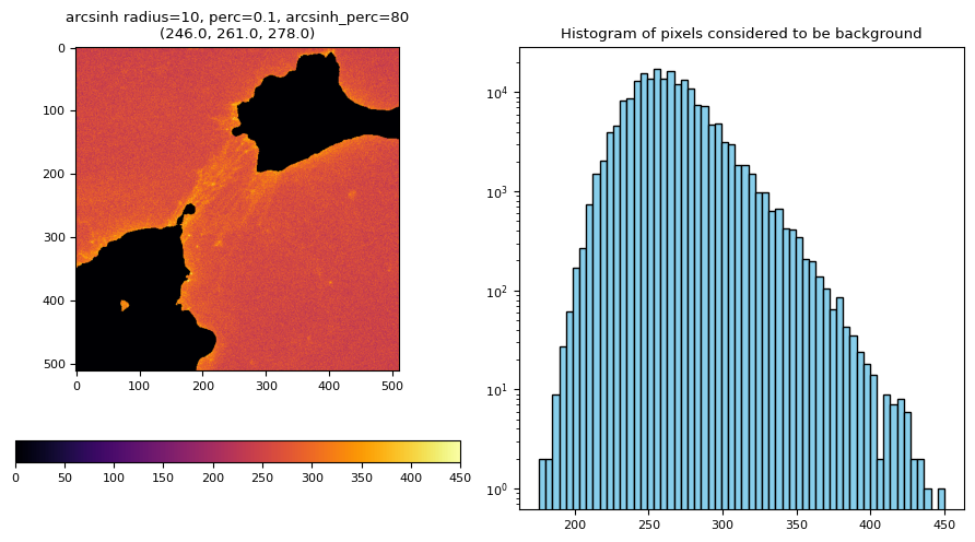
utils.bg(daimg[0, 0].compute())
(np.float64(457.8380994040984), np.float64(48.50287340564226))
def dabg(daimg):
r = defaultdict(list)
n_t, n_c = daimg.shape[:2]
for t in range(n_t):
for c in range(n_c):
r[c].append(utils.bg(daimg[t, c].compute())[0])
return pd.DataFrame(r)
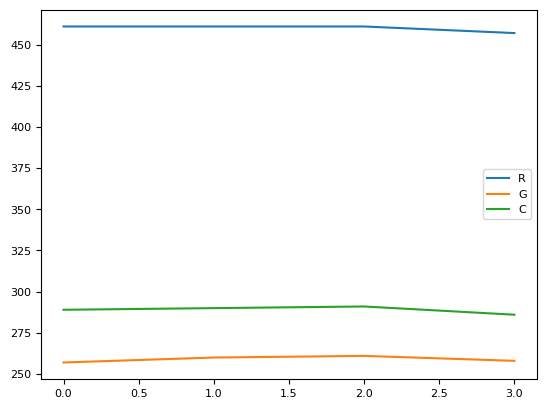
dabg(daimg)
| 0 | 1 | 2 | |
|---|---|---|---|
| 0 | 457.838099 | 257.010244 | 289.378226 |
| 1 | 457.295254 | 259.072941 | 289.627118 |
| 2 | 457.760167 | 260.182049 | 290.268666 |
| 3 | 453.995203 | 257.189940 | 285.613624 |
def dabg_fg(daimg, erf_pvalue=1e-100, size=10):
n_t, n_c = daimg.shape[:2]
bgs = defaultdict(list)
fgs = defaultdict(list)
for t in range(n_t):
p = np.ones(daimg.shape[-2:])
multichannel = daimg[t].compute()
for c in range(n_c):
av, sd = utils.bg(multichannel[c])
p *= utils.prob(multichannel[c], av, sd)
bgs[c].append(av)
mask = ndimage.median_filter((p) ** (1 / n_c), size=size) < erf_pvalue
for c in range(n_c):
fgs[c].append(np.ma.mean(np.ma.masked_array(multichannel[c], mask=~mask)))
return pd.DataFrame(bgs), pd.DataFrame(fgs)
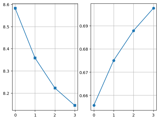
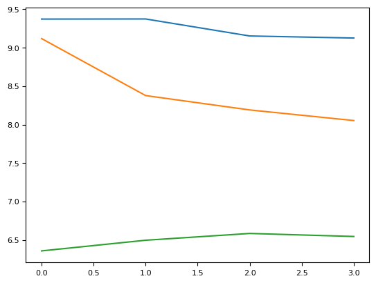
dfb, dff = dabg_fg(daimg)
plt.subplot(121)
((dff - dfb)[0] / (dff - dfb)[2]).plot(marker="s")
plt.grid()
plt.subplot(122)
((dff - dfb)[2] / (dff - dfb)[1]).plot(marker="o")
plt.grid()
NEXT:
make utils.bg and utils.prob work with dask arrays
def dmask(daim, erf_pvalue=1e-100, size=10):
n_c = daim.shape[0]
im = daim[0].compute()
p = utils.prob(im, *utils.bg(im))
for c in range(1, n_c):
im = daim[c].compute()
p *= utils.prob(im, *utils.bg(im))
p = ndimage.median_filter((p) ** (1 / n_c), size=size)
mask = p < erf_pvalue
return skimage.morphology.remove_small_objects(mask)
# mask = skimage.morphology.remove_small_holes(mask)
# return np.ma.masked_array(plane, mask=~mask), np.ma.masked_array(plane, mask=mask)
mask = dmask(daimg[2])
lab, nlab = ndimage.label(mask)
lab, nlab
(array([[0, 0, 0, ..., 0, 0, 0],
[0, 0, 0, ..., 0, 0, 0],
[0, 0, 0, ..., 0, 0, 0],
...,
[0, 0, 0, ..., 0, 0, 0],
[0, 0, 0, ..., 0, 0, 0],
[0, 0, 0, ..., 0, 0, 0]], shape=(512, 512), dtype=int32),
2)
pr = skimage.measure.regionprops(lab, intensity_image=daimg[0][0])
pr[1].equivalent_diameter_area
np.float64(195.49311541527658)
max_diameter = pr[0].equivalent_diameter_area
size = int(max_diameter * 0.3)
size
47
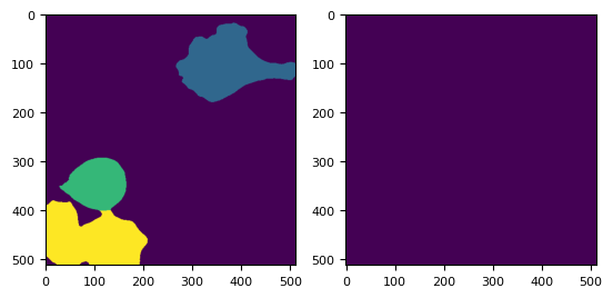
t = 0
mask = dmask(daimg[t])
# skimage.io.imshow(mask)
lab, nlab = ndimage.label(mask)
distance = ndimage.distance_transform_edt(mask)
# distance = skimage.filters.gaussian(distance, sigma=0) min_distance=size,
coords = skimage.feature.peak_local_max(
distance, footprint=np.ones((size, size)), labels=lab
)
mm = np.zeros(distance.shape, dtype=bool)
mm[tuple(coords.T)] = True
# markers, _ = ndimage.label(mm)
markers = skimage.measure.label(mm)
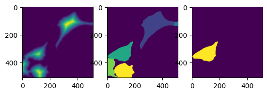
labels = skimage.segmentation.watershed(-distance, markers, mask=mask)
_, (ax0, ax1, ax2) = plt.subplots(1, 3)
ax0.imshow(distance)
ax1.imshow(labels)
ax2.imshow(labels == 3)
coords
array([[122, 329],
[122, 510],
[475, 125],
[341, 116],
[421, 1]])
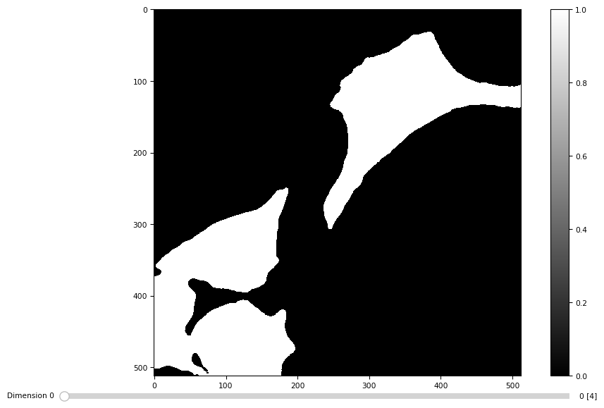
masks = [dmask(daimg[t]) for t in range(4)]
masks = np.stack(masks)
masks.shape
(4, 512, 512)
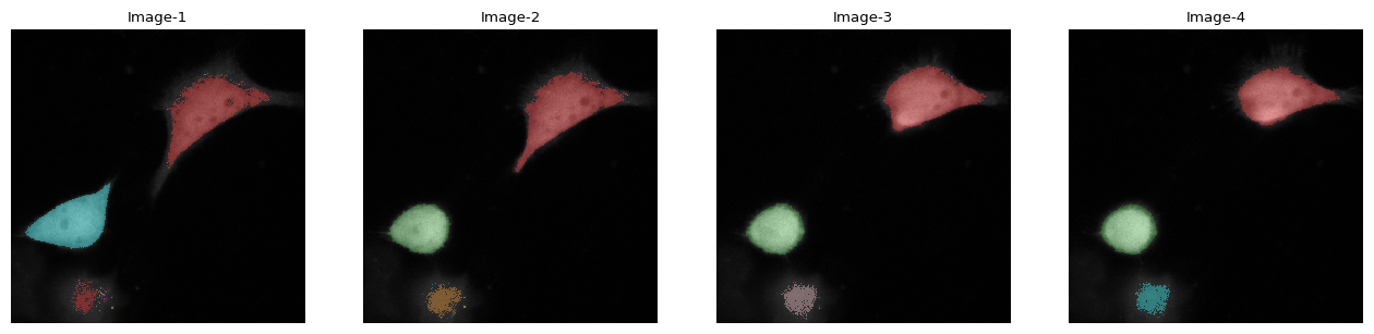
tff.imshow(masks)
(<Figure size 988.8x604.8 with 3 Axes>,
<Axes: >,
<matplotlib.image.AxesImage at 0x7fceb6050050>)
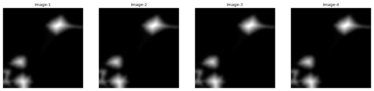
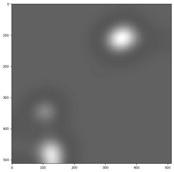
distance = ndimage.distance_transform_edt(masks)
distance = skimage.filters.gaussian(distance, sigma=5)
import impy
impy.array(distance).imshow()
| name | No name |
| shape | 4(t), 512(y), 512(x) |
| label shape | No label |
| dtype | float64 |
| source | None |
| scale | ScaleView(t=1.0000, y=1.0000, x=1.0000) |
for t in range(4):
coords = skimage.feature.peak_local_max(distance[t], footprint=np.ones((130, 130)))
print(coords)
[[114 346]
[473 128]
[344 110]]
[[114 346]
[473 128]
[344 110]]
[[114 346]
[473 128]
[344 110]]
[[114 346]
[473 128]
[344 110]]
co = np.stack([coords, coords, coords, coords])
coords.T
array([[114, 473, 344],
[346, 128, 110]])
mm = np.zeros(masks[0].shape, dtype=bool)
mm[tuple(co.T)] = True
# markers, _ = ndimage.label(mm)
markers = skimage.measure.label(np.stack([mm, mm, mm, mm]))
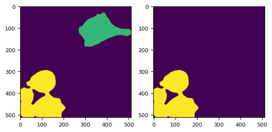
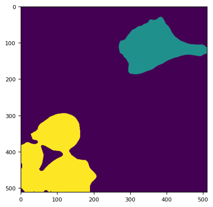
labels = skimage.segmentation.watershed(-distance, markers, mask=masks)
_, (ax1, ax2) = plt.subplots(1, 2)
ax1.imshow(labels[3])
ax2.imshow(labels[3] == 4)
<matplotlib.image.AxesImage at 0x7fceb4624690>
img = tff.imread(fp)
dim = io.read_image(fp, channels=["R", "G", "C"])
/home/runner/work/nima/nima/src/nima/io.py:53: UserWarning: Channel wavelength validation failed: Expected λ_C < λ_G < λ_R. Got C=458.0nm, G=563.0nm, R=482.0nm.
return nio.read_image(str(fp), channels=channels)
bg_params = nima.BgParams()
res = nima.bg(dim, bg_params)
bgs = res[1]
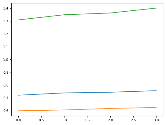
def ratio(t, roi):
if not np.any(labels[t] == roi):
return np.nan, np.nan
g = img[t, 0][labels[t] == roi].mean() - bgs["G"][t]
r = img[t, 1][labels[t] == roi].mean() - bgs["R"][t]
c = img[t, 2][labels[t] == roi].mean() - bgs["C"][t]
return g / c, c / r
ratio(1, 4)
(nan, nan)
rph = defaultdict(list)
rcl = defaultdict(list)
for roi in range(1, 5):
for t in range(4):
ph, cl = ratio(t, roi)
rph[roi].append(ph)
rcl[roi].append(cl)
plt.plot(rph[1])
plt.plot(rph[2])
plt.plot(rph[3])
plt.plot(rph[4])
[<matplotlib.lines.Line2D at 0x7fcea0d617f0>]
plt.plot(rcl[1])
plt.plot(rcl[2])
plt.plot(rcl[3])
plt.plot(rcl[4])
[<matplotlib.lines.Line2D at 0x7fcea0dceba0>]
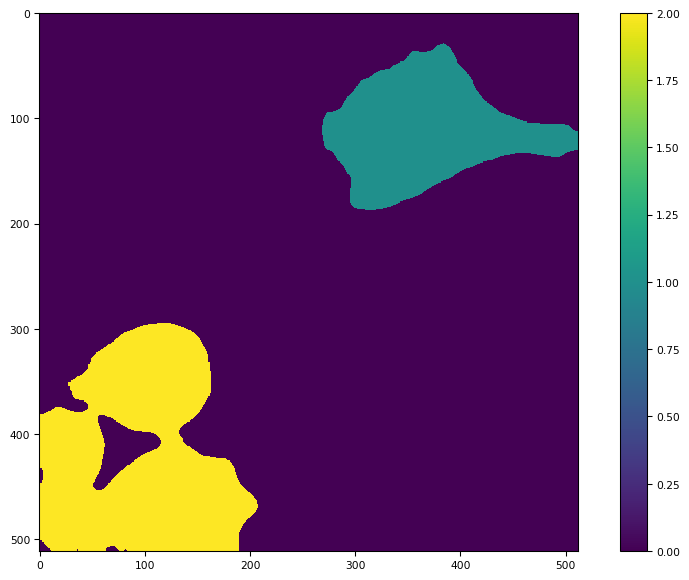
t = 2
mask = dmask(daimg[t])
# skimage.io.imshow(mask)
lab, nlab = ndimage.label(mask)
lab[~mask] = -1
# lab[lab==1] = -1
if np.any(lab == 0):
labels_ws = skimage.segmentation.random_walker(
daimg[t, 1].compute(), lab, beta=1e10, mode="bf"
)
else:
labels_ws = lab
# labels_ws = skimage.segmentation.random_walker(-distance, lab, beta=10000, mode="bf")
_, (ax1, ax2) = plt.subplots(1, 2)
ax1.imshow(labels_ws)
ax2.imshow(labels_ws == 2)
<matplotlib.image.AxesImage at 0x7fcead2e74d0>
imar = impy.imread(fp)
imar.label_threshold()
| name | 1b_c16_15.tif |
| shape | 4(t), 3(c), 512(y), 512(x) |
| dtype | uint16 |
| source | ../../tests/data/1b_c16_15.tif |
| scale | ScaleView(t=1.0000, c=1.0000, y=0.2000, x=0.2000) |
imar[:, 2].imshow(label=1)
| name | 1b_c16_15.tif |
| shape | 4(t), 512(y), 512(x) |
| label shape | 4(t), 512(y), 512(x) |
| dtype | uint16 |
| source | ../../tests/data/1b_c16_15.tif |
| scale | ScaleView(t=1.0000, y=0.2000, x=0.2000) |
def dmask0(im, erf_pvalue=1e-100, size=10):
p = utils.prob(im[0], *utils.bg(im[0]))
for img in im[1:]:
p *= utils.prob(img, *utils.bg(img))
p = ndimage.median_filter((p) ** (1 / len(im)), size=size)
mask = p < erf_pvalue
return skimage.morphology.remove_small_objects(mask)
dmask0(imar[1])
array([[False, False, False, ..., False, False, False],
[False, False, False, ..., False, False, False],
[False, False, False, ..., False, False, False],
...,
[False, False, False, ..., False, False, False],
[False, False, False, ..., False, False, False],
[False, False, False, ..., False, False, False]], shape=(512, 512))
plt.imshow(skimage.measure.label(mask))
<matplotlib.image.AxesImage at 0x7fcead39d810>
distance = skimage.filters.gaussian(distance, sigma=30)
tff.imshow(distance)
(<Figure size 988.8x604.8 with 1 Axes>,
<Axes: >,
<matplotlib.image.AxesImage at 0x7fcead34f250>)
np.transpose(np.nonzero(skimage.morphology.local_maxima(distance)))
array([[ 3, 110, 353],
[ 3, 346, 107],
[ 3, 456, 18],
[ 3, 486, 128]])
tff.imshow(ndimage.label(mask)[0])
(<Figure size 988.8x604.8 with 2 Axes>,
<Axes: >,
<matplotlib.image.AxesImage at 0x7fcead29a850>)
res[1]
| R | G | C | |
|---|---|---|---|
| 0 | 461.0 | 257.0 | 289.0 |
| 1 | 461.0 | 260.0 | 290.0 |
| 2 | 461.0 | 261.0 | 291.0 |
| 3 | 457.0 | 258.0 | 286.0 |
res[2]["G"][2][0]
res[1].plot()
<Axes: >
res[1].hvplot()
xim = dim
xim.data
|
||||||||||||||||
xim.coords["Y"]
<xarray.DataArray 'Y' (Y: 512)> Size: 4kB array([ 0. , 0.2, 0.4, ..., 101.8, 102. , 102.2], shape=(512,)) Coordinates: * Y (Y) float64 4kB 0.0 0.2 0.4 0.6 0.8 ... 101.6 101.8 102.0 102.2
xarray.DataArray
'Y'
- Y: 512
- 0.0 0.2 0.4 0.6 0.8 1.0 1.2 ... 101.2 101.4 101.6 101.8 102.0 102.2
array([ 0. , 0.2, 0.4, ..., 101.8, 102. , 102.2], shape=(512,))
- Y(Y)float640.0 0.2 0.4 ... 101.8 102.0 102.2
array([ 0. , 0.2, 0.4, ..., 101.8, 102. , 102.2], shape=(512,))
xim.sel(C="G")[1, 0].hvplot(width=400, height=300)
xim[0, :, 0].hvplot(
width=300,
subplots=True,
by="C",
)
hvplot.extension(
"bokeh",
"matplotlib",
)
img = xim.sel(C="R")[0][0]
hvimg = hv.Image(img)
hvimg
# %%opts Image [aspect=1388/1038]
f = xim.sel(C="R")[:, 0].hvplot(
frame_width=300,
frame_height=200,
subplots=True,
col="T",
yaxis=False,
colorbar=False,
xaxis=False,
cmap="Reds",
) + xim.sel(C="C")[:, 0].hvplot(
subplots=True, col="T", yaxis=False, colorbar=False, xaxis=False, cmap="Greens"
)
f
import bioio
bioio.__version__
'3.3.0'
hv.opts.defaults(
hv.opts.Image(aspect=1388 / 1038),
hv.opts.Image("Cyan", cmap=plt.cm.Blues),
hv.opts.Image("Green", cmap=plt.cm.Greens),
hv.opts.Image("Red", cmap=plt.cm.Reds),
)
dim.sel(C="C", Z=0)
<xarray.DataArray 'transpose-f90a051fb26499132bdac5e5b2db5a9d' (T: 4, Y: 512,
X: 512)> Size: 2MB
dask.array<getitem, shape=(4, 512, 512), dtype=uint16, chunksize=(1, 512, 512), chunktype=numpy.ndarray>
Coordinates:
* T (T) float64 32B 13.38 73.38 133.4 193.4
* Y (Y) float64 4kB 0.0 0.2 0.4 0.6 0.8 ... 101.6 101.8 102.0 102.2
* X (X) float64 4kB 0.0 0.2 0.4 0.6 0.8 ... 101.6 101.8 102.0 102.2
Z float64 8B 0.0
C <U1 4B 'C'
Attributes:
unprocessed: {254: <FILETYPE.PAGE: 2>, 256: 512, 257: 512, 258: 16, 259...
processed: experiments=[{'description': '', 'experimenter_ref': {'id'...
metadata: Metadata(S=1, T=[4], C=[3], Z=[1], Y=[512], X=[512]\n bit...
ome_metadata: experiments=[{'description': '', 'experimenter_ref': {'id'...xarray.DataArray
'transpose-f90a051fb26499132bdac5e5b2db5a9d'
- T: 4
- Y: 512
- X: 512
- dask.array<chunksize=(1, 512, 512), meta=np.ndarray>
Array Chunk Bytes 2.00 MiB 512.00 kiB Shape (4, 512, 512) (1, 512, 512) Dask graph 4 chunks in 45 graph layers Data type uint16 numpy.ndarray - T(T)float6413.38 73.38 133.4 193.4
array([ 13.38269, 73.38346, 133.3842 , 193.385 ])
- Y(Y)float640.0 0.2 0.4 ... 101.8 102.0 102.2
array([ 0. , 0.2, 0.4, ..., 101.8, 102. , 102.2], shape=(512,))
- X(X)float640.0 0.2 0.4 ... 101.8 102.0 102.2
array([ 0. , 0.2, 0.4, ..., 101.8, 102. , 102.2], shape=(512,))
- Z()float640.0
array(0.)
- C()<U1'C'
array('C', dtype='<U1')
- unprocessed :
- {254: <FILETYPE.PAGE: 2>, 256: 512, 257: 512, 258: 16, 259: <COMPRESSION.NONE: 1>, 262: <PHOTOMETRIC.MINISBLACK: 1>, 266: <FILLORDER.MSB2LSB: 1>, 270: '<?xml version = "1.0"?><OME xmlns="http://www.openmicroscopy.org/Schemas/OME/2013-06" xmlns:xsi="http://www.w3.org/2001/XMLSchema-instance" xmlns:OME="http://www.openmicroscopy.org/Schemas/OME/2013-06" xmlns:BIN="http://www.openmicroscopy.org/Schemas/BinaryFile/2013-06" xmlns:SPW="http://www.openmicroscopy.org/Schemas/SPW/2013-06" xmlns:SA="http://www.openmicroscopy.org/Schemas/SA/2013-06" xmlns:ROI="http://www.openmicroscopy.org/Schemas/ROI/2013-06" xsi:schemaLocation="http://www.openmicroscopy.org/Schemas/OME/2013-06 http://www.openmicroscopy.org/Schemas/OME/2013-06/ome.xsd http://www.openmicroscopy.org/Schemas/BinaryFile/2013-06 http://www.openmicroscopy.org/Schemas/BinaryFile/2013-06/BinaryFile.xsd http://www.openmicroscopy.org/Schemas/SPW/2013-06 http://www.openmicroscopy.org/Schemas/SPW/2013-06/SPW.xsd http://www.openmicroscopy.org/Schemas/SA/2013-06 http://www.openmicroscopy.org/Schemas/SA/2013-06/SA.xsd http://www.openmicroscopy.org/Schemas/ROI/2013-06 http://www.openmicroscopy.org/Schemas/ROI/2013-06/ROI.xsd" Creator="FEI Munich GmbH, Live Acquisition, V2.5.0.6"><OME:Experiment Type="FourDPlus" ID="Experiment:b43ba9de-c7fc-4cfb-a600-4cddf0f667ff"><OME:Description></OME:Description><OME:ExperimenterRef ID="Experimenter:41dab16c-9d73-42f9-896a-25fb785d8284" /></OME:Experiment><SPW:Plate ID="Plate:213b2240-4b81-4aac-aa8b-41b3c4b1ea24" Name="invitrogen_well" ColumnNamingConvention="number" RowNamingConvention="letter" Rows="1" Columns="1"><SPW:Description>PetriDish 6.51103101880453mm BorderTL: 0; 0mm BorderBR: 0; 0mm</SPW:Description><SPW:Well ID="Well:A1" Column="0" Row="0" /></SPW:Plate><OME:Experimenter ID="Experimenter:41dab16c-9d73-42f9-896a-25fb785d8284" /><OME:Instrument ID="Instrument:701dc90b-f5ce-4473-9232-e0681d402f29"><OME:Microscope Type="Inverted" Manufacturer="FEI Munich" Model="iMIC with Imaging Control Unit" /><OME:LightSource ID="LightSource:e8e7e8b2-30bd-4b3d-9162-d8193876d7fd_0" Power="150" Manufacturer="FEI Munich" Model="Oligochrome_0"><OME:Arc Type="Xe" /></OME:LightSource><OME:LightSource ID="LightSource:e8e7e8b2-30bd-4b3d-9162-d8193876d7fd_1" Power="150" Manufacturer="FEI Munich" Model="Oligochrome_1"><OME:Arc Type="Xe" /></OME:LightSource><OME:LightSource ID="LightSource:e8e7e8b2-30bd-4b3d-9162-d8193876d7fd_2" Power="150" Manufacturer="FEI Munich" Model="Oligochrome_2"><OME:Arc Type="Xe" /></OME:LightSource><OME:LightSource ID="LightSource:e8e7e8b2-30bd-4b3d-9162-d8193876d7fd_3" Power="150" Manufacturer="FEI Munich" Model="Oligochrome_3"><OME:Arc Type="Xe" /></OME:LightSource><OME:LightSource ID="LightSource:e8e7e8b2-30bd-4b3d-9162-d8193876d7fd_4" Power="150" Manufacturer="FEI Munich" Model="Oligochrome_4"><OME:Arc Type="Xe" /></OME:LightSource><OME:LightSource ID="LightSource:bf1d29d2-598f-4c8c-a3b8-efdeb6bca772" Manufacturer="FEI Munich" Model="LED"><OME:LightEmittingDiode /></OME:LightSource><OME:Detector ID="Detector:7ed7084b-6556-4638-a299-f3f679486e39" Type="CCD" Manufacturer="Andor" Model="Andor Ultra 897" /><OME:Detector ID="Detector:6eb646d5-7f50-4382-ae3e-1c0e6bada86e" Type="CCD" Manufacturer="Allied Vision Tech." Model="AVT Stingray F145B-30fps" /><OME:Objective ID="Objective:10XAir:d8a6fc21-dc73-4b6a-a8fb-1485a469d987" Manufacturer="Unknown" Model="Unknown" Immersion="Air" LensNA="0.4" NominalMagnification="10" CalibratedMagnification="10" /><OME:Objective ID="Objective:60XWater:70e0fa2f-409a-4925-a0b7-e64cbd9dd4f1" Manufacturer="Unknown" Model="Unknown" Immersion="Water" LensNA="1.2" NominalMagnification="60" CalibratedMagnification="60" /><OME:Objective ID="Objective:60XOil:a613c56e-8f5b-4658-b409-31487ee51ce0" Manufacturer="Unknown" Model="Unknown" Immersion="Oil" LensNA="1.49" NominalMagnification="60" CalibratedMagnification="60" /><OME:Objective ID="Objective:40XAir:98d60bc6-9e23-42a9-a645-f3b26655a087" Manufacturer="Unknown" Model="Unknown" Immersion="Air" LensNA="0.65" NominalMagnification="40" CalibratedMagnification="40" /><OME:Filter ID="Filter:8465a0e3-dd9d-4b0c-9af5-08c6f5964e56" Manufacturer="Unknown" Model="TIRF 488" /><OME:Filter ID="Filter:c3c1cf97-8f5f-4160-a117-59367da3b357" Manufacturer="Unknown" Model="Quadband 405/488/561/640" /><OME:Filter ID="Filter:2c42d929-eed2-4170-9bc9-57fb880882ff" Manufacturer="Unknown" Model="Dualband" /><OME:Filter ID="Filter:acd87abf-33bf-4585-8bf2-6b192aa7bf59" Manufacturer="Unknown" Model="Widefield" /><OME:Filter ID="Filter:9792ed8a-e27b-4328-9b78-1e3ccd619157" Manufacturer="Unknown" Model="CFP/YFP" /><OME:Filter ID="Filter:14958812-32c4-423d-a84f-d0bbcdccea80" Manufacturer="Unknown" Model="495DC" /><OME:Filter ID="Filter:3751703f-9a5a-4073-906e-640a131d12ce" Manufacturer="Unknown" Model="560DC" /><OME:Filter ID="Filter:ac2e87f4-0bca-4c1d-885a-9b03bed6b855" Manufacturer="Unknown" Model="Pos1" /><OME:Filter ID="Filter:bc993ab0-2fc1-4041-9051-8b8ca3428af7" Manufacturer="Unknown" Model="Pos2" /><OME:Filter ID="Filter:a4c1a568-eafb-4777-8c0b-8190ba232026" Manufacturer="Unknown" Model="Pos3" /></OME:Instrument><OME:Image ID="Image:240b0ea1-8a20-4c8f-8aac-75c6f4333864"><OME:AcquisitionDate>2015-01-26T14:22:49</OME:AcquisitionDate><OME:InstrumentRef ID="Instrument:701dc90b-f5ce-4473-9232-e0681d402f29" /><OME:ObjectiveSettings ID="Objective:40XAir:98d60bc6-9e23-42a9-a645-f3b26655a087" /><OME:StageLabel Name="FEI Munich Big Stage" X="0" Y="0" /><OME:Pixels ID="Pixels:1-0" DimensionOrder="XYZCT" Type="uint16" SizeX="512" SizeY="512" SizeZ="1" SizeC="3" SizeT="4" PhysicalSizeX="0.2" PhysicalSizeY="0.2" PhysicalSizeZ="1000" SignificantBits="16"><OME:Channel ID="Channel:0:e18c1bc2-9544-4c9c-a3a0-66835e0833c8" IlluminationType="Epifluorescence" AcquisitionMode="WideField"><OME:LightSourceSettings ID="LightSource:e8e7e8b2-30bd-4b3d-9162-d8193876d7fd_1" Attenuation="0.9" Wavelength="482" /><OME:DetectorSettings ID="Detector:7ed7084b-6556-4638-a299-f3f679486e39" Gain="50" Binning="1x1" /><OME:LightPath><OME:ExcitationFilterRef ID="Filter:2c42d929-eed2-4170-9bc9-57fb880882ff" /><OME:ExcitationFilterRef ID="Filter:acd87abf-33bf-4585-8bf2-6b192aa7bf59" /><OME:ExcitationFilterRef ID="Filter:ac2e87f4-0bca-4c1d-885a-9b03bed6b855" /></OME:LightPath></OME:Channel><OME:Channel ID="Channel:1:59761cf0-5b29-4dfa-a3dc-d2cb9740945e" IlluminationType="Epifluorescence" AcquisitionMode="WideField"><OME:LightSourceSettings ID="LightSource:e8e7e8b2-30bd-4b3d-9162-d8193876d7fd_2" Attenuation="0.9" Wavelength="563" /><OME:DetectorSettings ID="Detector:7ed7084b-6556-4638-a299-f3f679486e39" Gain="50" Binning="1x1" /><OME:LightPath><OME:ExcitationFilterRef ID="Filter:2c42d929-eed2-4170-9bc9-57fb880882ff" /><OME:ExcitationFilterRef ID="Filter:acd87abf-33bf-4585-8bf2-6b192aa7bf59" /><OME:ExcitationFilterRef ID="Filter:ac2e87f4-0bca-4c1d-885a-9b03bed6b855" /></OME:LightPath></OME:Channel><OME:Channel ID="Channel:2:97688b8f-c038-4ddc-8123-dac309db6bbd" IlluminationType="Epifluorescence" AcquisitionMode="WideField"><OME:LightSourceSettings ID="LightSource:e8e7e8b2-30bd-4b3d-9162-d8193876d7fd_4" Attenuation="0.9" Wavelength="458" /><OME:DetectorSettings ID="Detector:7ed7084b-6556-4638-a299-f3f679486e39" Gain="50" Binning="1x1" /><OME:LightPath><OME:ExcitationFilterRef ID="Filter:2c42d929-eed2-4170-9bc9-57fb880882ff" /><OME:ExcitationFilterRef ID="Filter:acd87abf-33bf-4585-8bf2-6b192aa7bf59" /><OME:ExcitationFilterRef ID="Filter:ac2e87f4-0bca-4c1d-885a-9b03bed6b855" /></OME:LightPath></OME:Channel><OME:TiffData IFD="0" FirstZ="0" FirstT="0" FirstC="0" /><OME:TiffData IFD="1" FirstZ="0" FirstT="0" FirstC="1" /><OME:TiffData IFD="2" FirstZ="0" FirstT="0" FirstC="2" /><OME:TiffData IFD="3" FirstZ="0" FirstT="1" FirstC="0" /><OME:TiffData IFD="4" FirstZ="0" FirstT="1" FirstC="1" /><OME:TiffData IFD="5" FirstZ="0" FirstT="1" FirstC="2" /><OME:TiffData IFD="6" FirstZ="0" FirstT="2" FirstC="0" /><OME:TiffData IFD="7" FirstZ="0" FirstT="2" FirstC="1" /><OME:TiffData IFD="8" FirstZ="0" FirstT="2" FirstC="2" /><OME:TiffData IFD="9" FirstZ="0" FirstT="3" FirstC="0" /><OME:TiffData IFD="10" FirstZ="0" FirstT="3" FirstC="1" /><OME:TiffData IFD="11" FirstZ="0" FirstT="3" FirstC="2" /><OME:Plane TheZ="0" TheT="0" TheC="0" DeltaT="12.33258" ExposureTime="0.5" PositionX="48.97899" PositionY="74.36727" PositionZ="21.3205" /><OME:Plane TheZ="0" TheT="0" TheC="1" DeltaT="12.85763" ExposureTime="0.5" PositionX="48.97899" PositionY="74.36727" PositionZ="21.3205" /><OME:Plane TheZ="0" TheT="0" TheC="2" DeltaT="13.38269" ExposureTime="0.5" PositionX="48.97899" PositionY="74.36727" PositionZ="21.3205" /><OME:Plane TheZ="0" TheT="1" TheC="0" DeltaT="72.33334" ExposureTime="0.5" PositionX="48.97899" PositionY="74.36727" PositionZ="21.3205" /><OME:Plane TheZ="0" TheT="1" TheC="1" DeltaT="72.8584" ExposureTime="0.5" PositionX="48.97899" PositionY="74.36727" PositionZ="21.3205" /><OME:Plane TheZ="0" TheT="1" TheC="2" DeltaT="73.38346" ExposureTime="0.5" PositionX="48.97899" PositionY="74.36727" PositionZ="21.3205" /><OME:Plane TheZ="0" TheT="2" TheC="0" DeltaT="132.3341" ExposureTime="0.5" PositionX="48.97899" PositionY="74.36727" PositionZ="21.3205" /><OME:Plane TheZ="0" TheT="2" TheC="1" DeltaT="132.8592" ExposureTime="0.5" PositionX="48.97899" PositionY="74.36727" PositionZ="21.3205" /><OME:Plane TheZ="0" TheT="2" TheC="2" DeltaT="133.3842" ExposureTime="0.5" PositionX="48.97899" PositionY="74.36727" PositionZ="21.3205" /><OME:Plane TheZ="0" TheT="3" TheC="0" DeltaT="192.3349" ExposureTime="0.5" PositionX="48.97899" PositionY="74.36727" PositionZ="21.3205" /><OME:Plane TheZ="0" TheT="3" TheC="1" DeltaT="192.8599" ExposureTime="0.5" PositionX="48.97899" PositionY="74.36727" PositionZ="21.3205" /><OME:Plane TheZ="0" TheT="3" TheC="2" DeltaT="193.385" ExposureTime="0.5" PositionX="48.97899" PositionY="74.36727" PositionZ="21.3205" /></OME:Pixels></OME:Image><SA:StructuredAnnotations><SA:XMLAnnotation ID="Annotation:e4967c06-941f-40a3-acd2-258c1d9012fa" Namespace="http://www.fei.com"><SA:Value><LA><LADisplayName Name="Arosio" /><AuxDevice Manufacturer="Unknown" Model="Computer" ID="Computer:BFEBFBFF000106A5" /><AuxDevice Manufacturer="FEI Munich" Model="Polytrope II with Yanus" ID="PolytropeIIYanus:37e223ba-eb29-4031-817d-8f870408fc77" /><AuxDevice Manufacturer="Unknown" Model="Hardware Autofocus" ID="HadrwareAutofocus:fd2cd8d8-4f29-429b-9287-e3c7085461ac" /><TubeRefractor CamID="Detector:7ed7084b-6556-4638-a299-f3f679486e39" Factor="2" /><TubeRefractor CamID="Detector:6eb646d5-7f50-4382-ae3e-1c0e6bada86e" Factor="1.002" /><FilterDeviceDescription ID="Microscope:a152ccd5-ebd9-49ac-b36e-8cbd478cf849" Name="iMIC with Imaging Control Unit"><FilterSliderDescription Index="0" Name="iMIC [Filters]"><FilterRef ID="Filter:8465a0e3-dd9d-4b0c-9af5-08c6f5964e56" /><FilterRef ID="Filter:c3c1cf97-8f5f-4160-a117-59367da3b357" /><FilterRef ID="Filter:2c42d929-eed2-4170-9bc9-57fb880882ff" /></FilterSliderDescription><FilterSliderDescription Index="1" Name="iMIC [Dichrotome]"><FilterRef ID="Filter:acd87abf-33bf-4585-8bf2-6b192aa7bf59" /><FilterRef ID="Filter:9792ed8a-e27b-4328-9b78-1e3ccd619157" /><FilterRef ID="Filter:14958812-32c4-423d-a84f-d0bbcdccea80" /><FilterRef ID="Filter:3751703f-9a5a-4073-906e-640a131d12ce" /></FilterSliderDescription><FilterSliderDescription Index="2" Name="iMIC [Filters]"><FilterRef ID="Filter:ac2e87f4-0bca-4c1d-885a-9b03bed6b855" /><FilterRef ID="Filter:bc993ab0-2fc1-4041-9051-8b8ca3428af7" /><FilterRef ID="Filter:a4c1a568-eafb-4777-8c0b-8190ba232026" /></FilterSliderDescription></FilterDeviceDescription><DeviceConnection FirstDeviceID="Computer:BFEBFBFF000106A5" FirstDevicePort="COM6" SecondDeviceID="Microscope:a152ccd5-ebd9-49ac-b36e-8cbd478cf849" SecondDevicePort="COM PORT" /><DeviceConnection FirstDeviceID="Computer:BFEBFBFF000106A5" FirstDevicePort="COM4" SecondDeviceID="PolytropeIIYanus:37e223ba-eb29-4031-817d-8f870408fc77" SecondDevicePort="COM PORT" /><DeviceConnection FirstDeviceID="Computer:BFEBFBFF000106A5" FirstDevicePort="COM3" SecondDeviceID="LightSource:e8e7e8b2-30bd-4b3d-9162-d8193876d7fd" SecondDevicePort="COM PORT" /><DeviceConnection FirstDeviceID="Microscope:a152ccd5-ebd9-49ac-b36e-8cbd478cf849" FirstDevicePort="SER 1" SecondDeviceID="PolytropeIIYanus:37e223ba-eb29-4031-817d-8f870408fc77" SecondDevicePort="COM PORT Axes" /><DeviceConnection FirstDeviceID="Microscope:a152ccd5-ebd9-49ac-b36e-8cbd478cf849" FirstDevicePort="Camera sync OUT" SecondDeviceID="Detector:7ed7084b-6556-4638-a299-f3f679486e39" SecondDevicePort="Trigger" /><DeviceConnection FirstDeviceID="Microscope:a152ccd5-ebd9-49ac-b36e-8cbd478cf849" FirstDevicePort="DO1" SecondDeviceID="PolytropeIIYanus:37e223ba-eb29-4031-817d-8f870408fc77" SecondDevicePort="Trigger In" /><DeviceConnection FirstDeviceID="Microscope:a152ccd5-ebd9-49ac-b36e-8cbd478cf849" FirstDevicePort="DO2" SecondDeviceID="LightSource:e8e7e8b2-30bd-4b3d-9162-d8193876d7fd" SecondDevicePort="TrigIn Cam" /><DeviceConnection FirstDeviceID="Microscope:a152ccd5-ebd9-49ac-b36e-8cbd478cf849" FirstDevicePort="Di1" SecondDeviceID="PolytropeIIYanus:37e223ba-eb29-4031-817d-8f870408fc77" SecondDevicePort="Trigger Out" /><DeviceConnection FirstDeviceID="Microscope:a152ccd5-ebd9-49ac-b36e-8cbd478cf849" FirstDevicePort="LED Trigger" SecondDeviceID="LightSource:bf1d29d2-598f-4c8c-a3b8-efdeb6bca772" SecondDevicePort="Trigger" /><DeviceConnection FirstDeviceID="Microscope:a152ccd5-ebd9-49ac-b36e-8cbd478cf849" FirstDevicePort="AO1" SecondDeviceID="HadrwareAutofocus:fd2cd8d8-4f29-429b-9287-e3c7085461ac" SecondDevicePort="Analog" /><DeviceConnection FirstDeviceID="Microscope:a152ccd5-ebd9-49ac-b36e-8cbd478cf849" FirstDevicePort="EIO1" SecondDeviceID="Detector:6eb646d5-7f50-4382-ae3e-1c0e6bada86e" SecondDevicePort="Trigger" /><DeviceConnection FirstDeviceID="Microscope:a152ccd5-ebd9-49ac-b36e-8cbd478cf849" FirstDevicePort="EIO2" SecondDeviceID="HadrwareAutofocus:fd2cd8d8-4f29-429b-9287-e3c7085461ac" SecondDevicePort="Trigger" /><FirmwareVersion ID="Microscope:a152ccd5-ebd9-49ac-b36e-8cbd478cf849" Version="FIRMWARE_3_5_32" Label="iMIC with Imaging Control Unit" /><FirmwareVersion ID="PolytropeIIYanus:37e223ba-eb29-4031-817d-8f870408fc77" Version="DSC: FIRMWARE_3_5_20 Compiled on: 2012-03-16 - 16-36" Label="Polytrope II with Yanus" /><FirmwareVersion ID="LightSource:e8e7e8b2-30bd-4b3d-9162-d8193876d7fd" Version="TILL Photonics Oligochrome 0 (firmware FIRMWARE_3_5_32)" Label="Oligochrome" /><FirmwareVersion ID="Detector:7ed7084b-6556-4638-a299-f3f679486e39" Version="USB; PCB: 28210, Decode: 7317, SerPar: 0, Clocks: 2, Camera: 6.17; EPROM: 0, COF: 0, Driver: 0.0, API: 2.94" Label="Andor Ultra 897" /><FirmwareVersion ID="Detector:6eb646d5-7f50-4382-ae3e-1c0e6bada86e" Version="MC: 00.01.09.04; FPGA: 00.02.01.07; API: 2.1.2.0" Label="AVT Stingray F145B-30fps" /><FRAPCalPoint XGalvo="-618475290.624" YGalvo="-1786706395.136" XPixel="264.929460580913" YPixel="245.131396957123" /><FRAPCalPoint XGalvo="3642132267.008" YGalvo="1786706395.136" XPixel="1126.91009681881" YPixel="179.858921161826" /><FRAPCalPoint XGalvo="618475290.624" YGalvo="5153960755.2" XPixel="1161.46611341632" YPixel="874.818810511757" /><PolytropeCal ParamName="none_angle" Position="-2.73851609230042" AuxDeviceRef="PolytropeIIYanus:37e223ba-eb29-4031-817d-8f870408fc77" /><PolytropeCal ParamName="epi_angle" Position="10.7799997329712" AuxDeviceRef="PolytropeIIYanus:37e223ba-eb29-4031-817d-8f870408fc77" /><PolytropeCal ParamName="tirf_angle" Position="-6.61126184463501" AuxDeviceRef="PolytropeIIYanus:37e223ba-eb29-4031-817d-8f870408fc77" /><PolytropeCal ParamName="frap_angle" Position="-16.6272506713867" AuxDeviceRef="PolytropeIIYanus:37e223ba-eb29-4031-817d-8f870408fc77" /><TIRFCalibration name="488 nm TIRF" objectiveDescr="60X NA 1.49" filterDescr="TIRF 488" laserWavelength="390" objectiveMagnification="40" objectiveNA="0.65" refractionOilGlass="1.518" refractionSample="1.337" yanusPresent="True" yanusCenterX="0.24" yanusCenterY="-0.54" lensPosition="9.18002449035645" alpha="90" offsetLeft="-0.576445952724299" offsetRight="-0.356445952724298" offsetTop="-0.636445952724299" offsetBottom="-0.266445952724299" useMainAxis="False" /><LAVersion Version="2.5.0.6" /><AxesDirections XInverted="true" YInverted="true" XYSwapped="true" ID="Microscope:a152ccd5-ebd9-49ac-b36e-8cbd478cf849" /><DisplayOrientation MirrorX="False" MirrorY="True" SwapXY="False" /><ChipWindow ChipX="0" ChipY="0" ChipWidth="512" ChipHeight="512" CamID="Detector:7ed7084b-6556-4638-a299-f3f679486e39" /><ChannelOverlayInfo OverlayActive="False" SplitActive="False" ChannelSplitLayout="4"><ChannelOverlaySingleVisibility ChannelIndex="0" Visible="True" /><ChannelOverlaySingleVisibility ChannelIndex="1" Visible="True" /><ChannelOverlaySingleVisibility ChannelIndex="2" Visible="True" /></ChannelOverlayInfo><LookUpTable ID="0" Name="Gray" ColorCount="1" ColorList="000000" DisplayMin="157" DisplayMax="1988" Autoscale="True" IgnoreMinPercent="0" IgnoreMaxPercent="0" SaturationMode="False" SaturationMinColor="0000FF" SaturationMaxColor="FF0000" /><LookUpTable ID="1" Name="Gray" ColorCount="1" ColorList="000000" DisplayMin="169" DisplayMax="1075" Autoscale="True" IgnoreMinPercent="0" IgnoreMaxPercent="0" SaturationMode="False" SaturationMinColor="0000FF" SaturationMaxColor="FF0000" /><LookUpTable ID="2" Name="Gray" ColorCount="1" ColorList="000000" DisplayMin="169" DisplayMax="1075" Autoscale="True" IgnoreMinPercent="0" IgnoreMaxPercent="0" SaturationMode="False" SaturationMinColor="0000FF" SaturationMaxColor="FF0000" /><ChannelOffsetInfo><SingleChannelOffset ChannelIndex="0" OverlapX="0" OverlapY="0" /><SingleChannelOffset ChannelIndex="1" OverlapX="0" OverlapY="0" /><SingleChannelOffset ChannelIndex="2" OverlapX="0" OverlapY="0" /></ChannelOffsetInfo><MultiChannelInfo ChannelIdx="0" MainLine="1"><MultiLineSingleInfo ID="LightSource:e8e7e8b2-30bd-4b3d-9162-d8193876d7fd_0" Attenuation="0" Wavelength="390" LineIndex="0" /><MultiLineSingleInfo ID="LightSource:e8e7e8b2-30bd-4b3d-9162-d8193876d7fd_2" Attenuation="0" Wavelength="563" LineIndex="2" /><MultiLineSingleInfo ID="LightSource:e8e7e8b2-30bd-4b3d-9162-d8193876d7fd_3" Attenuation="0" Wavelength="640" LineIndex="3" /><MultiLineSingleInfo ID="LightSource:e8e7e8b2-30bd-4b3d-9162-d8193876d7fd_4" Attenuation="0" Wavelength="458" LineIndex="4" /></MultiChannelInfo><MultiChannelInfo ChannelIdx="1" MainLine="2"><MultiLineSingleInfo ID="LightSource:e8e7e8b2-30bd-4b3d-9162-d8193876d7fd_0" Attenuation="0" Wavelength="390" LineIndex="0" /><MultiLineSingleInfo ID="LightSource:e8e7e8b2-30bd-4b3d-9162-d8193876d7fd_1" Attenuation="0" Wavelength="482" LineIndex="1" /><MultiLineSingleInfo ID="LightSource:e8e7e8b2-30bd-4b3d-9162-d8193876d7fd_3" Attenuation="0" Wavelength="640" LineIndex="3" /><MultiLineSingleInfo ID="LightSource:e8e7e8b2-30bd-4b3d-9162-d8193876d7fd_4" Attenuation="0" Wavelength="458" LineIndex="4" /></MultiChannelInfo><MultiChannelInfo ChannelIdx="2" MainLine="4"><MultiLineSingleInfo ID="LightSource:e8e7e8b2-30bd-4b3d-9162-d8193876d7fd_0" Attenuation="0" Wavelength="390" LineIndex="0" /><MultiLineSingleInfo ID="LightSource:e8e7e8b2-30bd-4b3d-9162-d8193876d7fd_1" Attenuation="0" Wavelength="482" LineIndex="1" /><MultiLineSingleInfo ID="LightSource:e8e7e8b2-30bd-4b3d-9162-d8193876d7fd_2" Attenuation="0" Wavelength="563" LineIndex="2" /><MultiLineSingleInfo ID="LightSource:e8e7e8b2-30bd-4b3d-9162-d8193876d7fd_3" Attenuation="0" Wavelength="640" LineIndex="3" /></MultiChannelInfo><LAProtocolRestore ExperimentName="Protocol Combination"><protocol_combination cultureInv="invariant">\r\n <Children>\r\n <count>1</count>\r\n <item_0 type="till.model.ProtocolAtomar, till.model, Version=1.0.0.0, Culture=neutral, PublicKeyToken=null">\r\n <Data type="till.model.ProtocolAtomar, till.model, Version=1.0.0.0, Culture=neutral, PublicKeyToken=null">\r\n <Name>Loop</Name>\r\n <Properties>\r\n <count>7</count>\r\n <item_0>\r\n <name>wellplate</name>\r\n <value type="System.Boolean, mscorlib, Version=2.0.0.0, Culture=neutral, PublicKeyToken=b77a5c561934e089">False</value>\r\n <Relative>False</Relative>\r\n <ForAnalysis>False</ForAnalysis>\r\n </item_0>\r\n <item_1>\r\n <name>global_coordinates</name>\r\n <value type="till.model.SerialList`1[[till.model.SerialList`1[[till.DoubleCoordinate, till, Version=1.0.0.0, Culture=neutral, PublicKeyToken=null]], till.model, Version=1.0.0.0, Culture=neutral, PublicKeyToken=null]], till.model, Version=1.0.0.0, Culture=neutral, PublicKeyToken=null">\r\n <count>1</count>\r\n <item_0>\r\n <count>0</count>\r\n </item_0>\r\n </value>\r\n <Relative>False</Relative>\r\n <ForAnalysis>False</ForAnalysis>\r\n </item_1>\r\n <item_2>\r\n <name>stage_coordinates</name>\r\n <value type="till.model.SerialList`1[[till.model.SerialList`1[[till.DoubleCoordinate, till, Version=1.0.0.0, Culture=neutral, PublicKeyToken=null]], till.model, Version=1.0.0.0, Culture=neutral, PublicKeyToken=null]], till.model, Version=1.0.0.0, Culture=neutral, PublicKeyToken=null">\r\n <count>1</count>\r\n <item_0>\r\n <count>0</count>\r\n </item_0>\r\n </value>\r\n <Relative>False</Relative>\r\n <ForAnalysis>False</ForAnalysis>\r\n </item_2>\r\n <item_3>\r\n <name>loop_count</name>\r\n <value type="System.Int32, mscorlib, Version=2.0.0.0, Culture=neutral, PublicKeyToken=b77a5c561934e089">40</value>\r\n <Relative>False</Relative>\r\n <ForAnalysis>False</ForAnalysis>\r\n </item_3>\r\n <item_4>\r\n <name>use_minimal_cycle</name>\r\n <value type="System.Boolean, mscorlib, Version=2.0.0.0, Culture=neutral, PublicKeyToken=b77a5c561934e089">False</value>\r\n <Relative>False</Relative>\r\n <ForAnalysis>False</ForAnalysis>\r\n </item_4>\r\n <item_5>\r\n <name>loop_cycle</name>\r\n <value type="System.Double, mscorlib, Version=2.0.0.0, Culture=neutral, PublicKeyToken=b77a5c561934e089">60000</value>\r\n <Relative>False</Relative>\r\n <ForAnalysis>False</ForAnalysis>\r\n </item_5>\r\n <item_6>\r\n <name>focus_clamp</name>\r\n <value type="System.Boolean, mscorlib, Version=2.0.0.0, Culture=neutral, PublicKeyToken=b77a5c561934e089">False</value>\r\n <Relative>False</Relative>\r\n <ForAnalysis>False</ForAnalysis>\r\n </item_6>\r\n </Properties>\r\n <CombineFile>False</CombineFile>\r\n <CombinationParameter>t</CombinationParameter>\r\n <AdditionalProperties>\r\n <count>0</count>\r\n </AdditionalProperties>\r\n </Data>\r\n <Children>\r\n <count>1</count>\r\n <item_0 type="till.model.ProtocolAtomar, till.model, Version=1.0.0.0, Culture=neutral, PublicKeyToken=null">\r\n <Data type="till.model.ProtocolAtomar, till.model, Version=1.0.0.0, Culture=neutral, PublicKeyToken=null">\r\n <Name>Marker Scan</Name>\r\n <Properties>\r\n <count>5</count>\r\n <item_0>\r\n <name>wellplate</name>\r\n <value type="System.Boolean, mscorlib, Version=2.0.0.0, Culture=neutral, PublicKeyToken=b77a5c561934e089">False</value>\r\n <Relative>False</Relative>\r\n <ForAnalysis>False</ForAnalysis>\r\n </item_0>\r\n <item_1>\r\n <name>global_coordinates</name>\r\n <value type="till.model.SerialList`1[[till.model.SerialList`1[[till.DoubleCoordinate, till, Version=1.0.0.0, Culture=neutral, PublicKeyToken=null]], till.model, Version=1.0.0.0, Culture=neutral, PublicKeyToken=null]], till.model, Version=1.0.0.0, Culture=neutral, PublicKeyToken=null">\r\n <count>1</count>\r\n <item_0>\r\n <count>0</count>\r\n </item_0>\r\n </value>\r\n <Relative>False</Relative>\r\n <ForAnalysis>False</ForAnalysis>\r\n </item_1>\r\n <item_2>\r\n <name>stage_coordinates</name>\r\n <value type="till.model.SerialList`1[[till.model.SerialList`1[[till.DoubleCoordinate, till, Version=1.0.0.0, Culture=neutral, PublicKeyToken=null]], till.model, Version=1.0.0.0, Culture=neutral, PublicKeyToken=null]], till.model, Version=1.0.0.0, Culture=neutral, PublicKeyToken=null">\r\n <count>1</count>\r\n <item_0>\r\n <count>0</count>\r\n </item_0>\r\n </value>\r\n <Relative>False</Relative>\r\n <ForAnalysis>False</ForAnalysis>\r\n </item_2>\r\n <item_3>\r\n <name>camera_independent</name>\r\n <value type="System.Boolean, mscorlib, Version=2.0.0.0, Culture=neutral, PublicKeyToken=b77a5c561934e089">True</value>\r\n <Relative>False</Relative>\r\n <ForAnalysis>False</ForAnalysis>\r\n </item_3>\r\n <item_4>\r\n <name>image_markers</name>\r\n <value type="till.model.SerialList`1[[till.model.ProtocolProperty, till.model, Version=1.0.0.0, Culture=neutral, PublicKeyToken=null]], till.model, Version=1.0.0.0, Culture=neutral, PublicKeyToken=null">\r\n <count>9</count>\r\n <item_0>\r\n <name>c3</name>\r\n <value type="till.model.SerialList`1[[System.Double, mscorlib, Version=2.0.0.0, Culture=neutral, PublicKeyToken=b77a5c561934e089]], till.model, Version=1.0.0.0, Culture=neutral, PublicKeyToken=null">\r\n <count>5</count>\r\n <item_0>80.7785085439682</item_0>\r\n <item_1>46.8039861222108</item_1>\r\n <item_2>21.3185</item_2>\r\n <item_3>0</item_3>\r\n <item_4>3</item_4>\r\n </value>\r\n <Relative>False</Relative>\r\n <ForAnalysis>False</ForAnalysis>\r\n </item_0>\r\n <item_1>\r\n <name>c5</name>\r\n <value type="till.model.SerialList`1[[System.Double, mscorlib, Version=2.0.0.0, Culture=neutral, PublicKeyToken=b77a5c561934e089]], till.model, Version=1.0.0.0, Culture=neutral, PublicKeyToken=null">\r\n <count>5</count>\r\n <item_0>80.4492950886488</item_0>\r\n <item_1>46.1306856373946</item_1>\r\n <item_2>21.318</item_2>\r\n <item_3>0</item_3>\r\n <item_4>3</item_4>\r\n </value>\r\n <Relative>False</Relative>\r\n <ForAnalysis>False</ForAnalysis>\r\n </item_1>\r\n <item_2>\r\n <name>c6</name>\r\n <value type="till.model.SerialList`1[[System.Double, mscorlib, Version=2.0.0.0, Culture=neutral, PublicKeyToken=b77a5c561934e089]], till.model, Version=1.0.0.0, Culture=neutral, PublicKeyToken=null">\r\n <count>5</count>\r\n <item_0>80.3048582673073</item_0>\r\n <item_1>46.1776553094387</item_1>\r\n <item_2>21.319</item_2>\r\n <item_3>0</item_3>\r\n <item_4>3</item_4>\r\n </value>\r\n <Relative>False</Relative>\r\n <ForAnalysis>False</ForAnalysis>\r\n </item_2>\r\n <item_3>\r\n <name>c8</name>\r\n <value type="till.model.SerialList`1[[System.Double, mscorlib, Version=2.0.0.0, Culture=neutral, PublicKeyToken=b77a5c561934e089]], till.model, Version=1.0.0.0, Culture=neutral, PublicKeyToken=null">\r\n <count>5</count>\r\n <item_0>80.0019134581089</item_0>\r\n <item_1>46.1865823368231</item_1>\r\n <item_2>21.321</item_2>\r\n <item_3>0</item_3>\r\n <item_4>3</item_4>\r\n </value>\r\n <Relative>False</Relative>\r\n <ForAnalysis>False</ForAnalysis>\r\n </item_3>\r\n <item_4>\r\n <name>c10</name>\r\n <value type="till.model.SerialList`1[[System.Double, mscorlib, Version=2.0.0.0, Culture=neutral, PublicKeyToken=b77a5c561934e089]], till.model, Version=1.0.0.0, Culture=neutral, PublicKeyToken=null">\r\n <count>5</count>\r\n <item_0>79.681098267436</item_0>\r\n <item_1>46.5777270893256</item_1>\r\n <item_2>21.319</item_2>\r\n <item_3>0</item_3>\r\n <item_4>3</item_4>\r\n </value>\r\n <Relative>False</Relative>\r\n <ForAnalysis>False</ForAnalysis>\r\n </item_4>\r\n <item_5>\r\n <name>c13</name>\r\n <value type="till.model.SerialList`1[[System.Double, mscorlib, Version=2.0.0.0, Culture=neutral, PublicKeyToken=b77a5c561934e089]], till.model, Version=1.0.0.0, Culture=neutral, PublicKeyToken=null">\r\n <count>5</count>\r\n <item_0>81.127021715045</item_0>\r\n <item_1>45.3031883736451</item_1>\r\n <item_2>21.3215</item_2>\r\n <item_3>0</item_3>\r\n <item_4>3</item_4>\r\n </value>\r\n <Relative>False</Relative>\r\n <ForAnalysis>False</ForAnalysis>\r\n </item_5>\r\n <item_6>\r\n <name>c15</name>\r\n <value type="till.model.SerialList`1[[System.Double, mscorlib, Version=2.0.0.0, Culture=neutral, PublicKeyToken=b77a5c561934e089]], till.model, Version=1.0.0.0, Culture=neutral, PublicKeyToken=null">\r\n <count>5</count>\r\n <item_0>80.3952395915985</item_0>\r\n <item_1>46.6838236351808</item_1>\r\n <item_2>21.321</item_2>\r\n <item_3>0</item_3>\r\n <item_4>3</item_4>\r\n </value>\r\n <Relative>False</Relative>\r\n <ForAnalysis>False</ForAnalysis>\r\n </item_6>\r\n <item_7>\r\n <name>c16</name>\r\n <value type="till.model.SerialList`1[[System.Double, mscorlib, Version=2.0.0.0, Culture=neutral, PublicKeyToken=b77a5c561934e089]], till.model, Version=1.0.0.0, Culture=neutral, PublicKeyToken=null">\r\n <count>5</count>\r\n <item_0>80.4829029589891</item_0>\r\n <item_1>46.3257147570451</item_1>\r\n <item_2>21.3205</item_2>\r\n <item_3>0</item_3>\r\n <item_4>3</item_4>\r\n </value>\r\n <Relative>False</Relative>\r\n <ForAnalysis>False</ForAnalysis>\r\n </item_7>\r\n <item_8>\r\n <name>c17</name>\r\n <value type="till.model.SerialList`1[[System.Double, mscorlib, Version=2.0.0.0, Culture=neutral, PublicKeyToken=b77a5c561934e089]], till.model, Version=1.0.0.0, Culture=neutral, PublicKeyToken=null">\r\n <count>5</count>\r\n <item_0>77.774062693119</item_0>\r\n <item_1>45.9996506770452</item_1>\r\n <item_2>21.319</item_2>\r\n <item_3>0</item_3>\r\n <item_4>3</item_4>\r\n </value>\r\n <Relative>False</Relative>\r\n <ForAnalysis>False</ForAnalysis>\r\n </item_8>\r\n </value>\r\n <Relative>False</Relative>\r\n <ForAnalysis>False</ForAnalysis>\r\n </item_4>\r\n </Properties>\r\n <CombineFile>False</CombineFile>\r\n <CombinationParameter>t</CombinationParameter>\r\n <AdditionalProperties>\r\n <count>0</count>\r\n </AdditionalProperties>\r\n </Data>\r\n <Children>\r\n <count>2</count>\r\n <item_0 type="till.model.ProtocolAtomar, till.model, Version=1.0.0.0, Culture=neutral, PublicKeyToken=null">\r\n <Data type="till.model.ProtocolAtomar, till.model, Version=1.0.0.0, Culture=neutral, PublicKeyToken=null">\r\n <Name>Multi Channels</Name>\r\n <Properties>\r\n <count>18</count>\r\n <item_0>\r\n <name>wellplate</name>\r\n <value type="System.Boolean, mscorlib, Version=2.0.0.0, Culture=neutral, PublicKeyToken=b77a5c561934e089">False</value>\r\n <Relative>False</Relative>\r\n <ForAnalysis>False</ForAnalysis>\r\n </item_0>\r\n <item_1>\r\n <name>global_coordinates</name>\r\n <value type="till.model.SerialList`1[[till.model.SerialList`1[[till.DoubleCoordinate, till, Version=1.0.0.0, Culture=neutral, PublicKeyToken=null]], till.model, Version=1.0.0.0, Culture=neutral, PublicKeyToken=null]], till.model, Version=1.0.0.0, Culture=neutral, PublicKeyToken=null">\r\n <count>1</count>\r\n <item_0>\r\n <count>0</count>\r\n </item_0>\r\n </value>\r\n <Relative>False</Relative>\r\n <ForAnalysis>False</ForAnalysis>\r\n </item_1>\r\n <item_2>\r\n <name>stage_coordinates</name>\r\n <value type="till.model.SerialList`1[[till.model.SerialList`1[[till.DoubleCoordinate, till, Version=1.0.0.0, Culture=neutral, PublicKeyToken=null]], till.model, Version=1.0.0.0, Culture=neutral, PublicKeyToken=null]], till.model, Version=1.0.0.0, Culture=neutral, PublicKeyToken=null">\r\n <count>1</count>\r\n <item_0>\r\n <count>0</count>\r\n </item_0>\r\n </value>\r\n <Relative>False</Relative>\r\n <ForAnalysis>False</ForAnalysis>\r\n </item_2>\r\n <item_3>\r\n <name>settings_count</name>\r\n <value type="System.Int32, mscorlib, Version=2.0.0.0, Culture=neutral, PublicKeyToken=b77a5c561934e089">3</value>\r\n <Relative>False</Relative>\r\n <ForAnalysis>False</ForAnalysis>\r\n </item_3>\r\n <item_4>\r\n <name>wave_experiment</name>\r\n <value type="System.Boolean, mscorlib, Version=2.0.0.0, Culture=neutral, PublicKeyToken=b77a5c561934e089">False</value>\r\n <Relative>False</Relative>\r\n <ForAnalysis>False</ForAnalysis>\r\n </item_4>\r\n <item_5>\r\n <name>light</name>\r\n <value type="System.String, mscorlib, Version=2.0.0.0, Culture=neutral, PublicKeyToken=b77a5c561934e089">Polychrome 3000</value>\r\n <Relative>False</Relative>\r\n <ForAnalysis>False</ForAnalysis>\r\n </item_5>\r\n <item_6>\r\n <name>exposure_is_dwell</name>\r\n <value type="System.Boolean, mscorlib, Version=2.0.0.0, Culture=neutral, PublicKeyToken=b77a5c561934e089">False</value>\r\n <Relative>False</Relative>\r\n <ForAnalysis>False</ForAnalysis>\r\n </item_6>\r\n <item_7>\r\n <name>polytrope_modus</name>\r\n <value type="till.model.POLYTROP_POS, till.model, Version=1.0.0.0, Culture=neutral, PublicKeyToken=null">EPI</value>\r\n <Relative>False</Relative>\r\n <ForAnalysis>False</ForAnalysis>\r\n </item_7>\r\n <item_8>\r\n <name>lines_count</name>\r\n <value type="System.Int32, mscorlib, Version=2.0.0.0, Culture=neutral, PublicKeyToken=b77a5c561934e089">5</value>\r\n <Relative>False</Relative>\r\n <ForAnalysis>False</ForAnalysis>\r\n </item_8>\r\n <item_9>\r\n <name>exposures</name>\r\n <value type="till.model.SerialList`1[[System.Double, mscorlib, Version=2.0.0.0, Culture=neutral, PublicKeyToken=b77a5c561934e089]], till.model, Version=1.0.0.0, Culture=neutral, PublicKeyToken=null">\r\n <count>3</count>\r\n <item_0>0.5</item_0>\r\n <item_1>0.5</item_1>\r\n <item_2>0.5</item_2>\r\n </value>\r\n <Relative>False</Relative>\r\n <ForAnalysis>False</ForAnalysis>\r\n </item_9>\r\n <item_10>\r\n <name>cycles</name>\r\n <value type="till.model.SerialList`1[[System.Double, mscorlib, Version=2.0.0.0, Culture=neutral, PublicKeyToken=b77a5c561934e089]], till.model, Version=1.0.0.0, Culture=neutral, PublicKeyToken=null">\r\n <count>3</count>\r\n <item_0>0.525</item_0>\r\n <item_1>0.525</item_1>\r\n <item_2>0.525</item_2>\r\n </value>\r\n <Relative>False</Relative>\r\n <ForAnalysis>False</ForAnalysis>\r\n </item_10>\r\n <item_11>\r\n <name>light_settings</name>\r\n <value type="till.model.SerialList`1[[till.model.SerialList`1[[System.Double, mscorlib, Version=2.0.0.0, Culture=neutral, PublicKeyToken=b77a5c561934e089]], till.model, Version=1.0.0.0, Culture=neutral, PublicKeyToken=null]], till.model, Version=1.0.0.0, Culture=neutral, PublicKeyToken=null">\r\n <count>3</count>\r\n <item_0>\r\n <count>5</count>\r\n <item_0>0</item_0>\r\n <item_1>90</item_1>\r\n <item_2>0</item_2>\r\n <item_3>0</item_3>\r\n <item_4>0</item_4>\r\n </item_0>\r\n <item_1>\r\n <count>5</count>\r\n <item_0>0</item_0>\r\n <item_1>0</item_1>\r\n <item_2>90</item_2>\r\n <item_3>0</item_3>\r\n <item_4>0</item_4>\r\n </item_1>\r\n <item_2>\r\n <count>5</count>\r\n <item_0>0</item_0>\r\n <item_1>0</item_1>\r\n <item_2>0</item_2>\r\n <item_3>0</item_3>\r\n <item_4>90</item_4>\r\n </item_2>\r\n </value>\r\n <Relative>False</Relative>\r\n <ForAnalysis>False</ForAnalysis>\r\n </item_11>\r\n <item_12>\r\n <name>filter_changes</name>\r\n <value type="till.model.SerialList`1[[till.model.SerialList`1[[till.model.FilterChange, till.model, Version=1.0.0.0, Culture=neutral, PublicKeyToken=null]], till.model, Version=1.0.0.0, Culture=neutral, PublicKeyToken=null]], till.model, Version=1.0.0.0, Culture=neutral, PublicKeyToken=null">\r\n <count>3</count>\r\n <item_0>\r\n <count>1</count>\r\n <item_0>\r\n <FilterChanger>\r\n <DeviceName>iMIC with Imaging Control Unit</DeviceName>\r\n <SliderIndex>0</SliderIndex>\r\n </FilterChanger>\r\n <FilterPosition>2</FilterPosition>\r\n </item_0>\r\n </item_0>\r\n <item_1>\r\n <count>1</count>\r\n <item_0>\r\n <FilterChanger>\r\n <DeviceName>iMIC with Imaging Control Unit</DeviceName>\r\n <SliderIndex>0</SliderIndex>\r\n </FilterChanger>\r\n <FilterPosition>2</FilterPosition>\r\n </item_0>\r\n </item_1>\r\n <item_2>\r\n <count>1</count>\r\n <item_0>\r\n <FilterChanger>\r\n <DeviceName>iMIC with Imaging Control Unit</DeviceName>\r\n <SliderIndex>0</SliderIndex>\r\n </FilterChanger>\r\n <FilterPosition>2</FilterPosition>\r\n </item_0>\r\n </item_2>\r\n </value>\r\n <Relative>False</Relative>\r\n <ForAnalysis>False</ForAnalysis>\r\n </item_12>\r\n <item_13>\r\n <name>focus_clamp</name>\r\n <value type="till.model.SerialList`1[[System.Boolean, mscorlib, Version=2.0.0.0, Culture=neutral, PublicKeyToken=b77a5c561934e089]], till.model, Version=1.0.0.0, Culture=neutral, PublicKeyToken=null">\r\n <count>3</count>\r\n <item_0>False</item_0>\r\n <item_1>False</item_1>\r\n <item_2>False</item_2>\r\n </value>\r\n <Relative>False</Relative>\r\n <ForAnalysis>False</ForAnalysis>\r\n </item_13>\r\n <item_14>\r\n <name>pre_loop_focus_clamp</name>\r\n <value type="System.Boolean, mscorlib, Version=2.0.0.0, Culture=neutral, PublicKeyToken=b77a5c561934e089">False</value>\r\n <Relative>False</Relative>\r\n <ForAnalysis>False</ForAnalysis>\r\n </item_14>\r\n <item_15>\r\n <name>total_cycle</name>\r\n <value type="System.Double, mscorlib, Version=2.0.0.0, Culture=neutral, PublicKeyToken=b77a5c561934e089">1.575</value>\r\n <Relative>False</Relative>\r\n <ForAnalysis>False</ForAnalysis>\r\n </item_15>\r\n <item_16>\r\n <name>repeat</name>\r\n <value type="System.Int32, mscorlib, Version=2.0.0.0, Culture=neutral, PublicKeyToken=b77a5c561934e089">1</value>\r\n <Relative>False</Relative>\r\n <ForAnalysis>False</ForAnalysis>\r\n </item_16>\r\n <item_17>\r\n <name>use_minimal_cycle</name>\r\n <value type="System.Boolean, mscorlib, Version=2.0.0.0, Culture=neutral, PublicKeyToken=b77a5c561934e089">True</value>\r\n <Relative>False</Relative>\r\n <ForAnalysis>False</ForAnalysis>\r\n </item_17>\r\n </Properties>\r\n <CombineFile>False</CombineFile>\r\n <CombinationParameter>t</CombinationParameter>\r\n <AdditionalProperties>\r\n <count>0</count>\r\n </AdditionalProperties>\r\n </Data>\r\n <Children>\r\n <count>0</count>\r\n </Children>\r\n </item_0>\r\n <item_1 type="till.model.ProtocolAtomar, till.model, Version=1.0.0.0, Culture=neutral, PublicKeyToken=null">\r\n <Data type="till.model.ProtocolAtomar, till.model, Version=1.0.0.0, Culture=neutral, PublicKeyToken=null">\r\n <Name>Single Snapshot</Name>\r\n <Properties>\r\n <count>13</count>\r\n <item_0>\r\n <name>wellplate</name>\r\n <value type="System.Boolean, mscorlib, Version=2.0.0.0, Culture=neutral, PublicKeyToken=b77a5c561934e089">False</value>\r\n <Relative>False</Relative>\r\n <ForAnalysis>False</ForAnalysis>\r\n </item_0>\r\n <item_1>\r\n <name>global_coordinates</name>\r\n <value type="till.model.SerialList`1[[till.model.SerialList`1[[till.DoubleCoordinate, till, Version=1.0.0.0, Culture=neutral, PublicKeyToken=null]], till.model, Version=1.0.0.0, Culture=neutral, PublicKeyToken=null]], till.model, Version=1.0.0.0, Culture=neutral, PublicKeyToken=null">\r\n <count>1</count>\r\n <item_0>\r\n <count>0</count>\r\n </item_0>\r\n </value>\r\n <Relative>False</Relative>\r\n <ForAnalysis>False</ForAnalysis>\r\n </item_1>\r\n <item_2>\r\n <name>stage_coordinates</name>\r\n <value type="till.model.SerialList`1[[till.model.SerialList`1[[till.DoubleCoordinate, till, Version=1.0.0.0, Culture=neutral, PublicKeyToken=null]], till.model, Version=1.0.0.0, Culture=neutral, PublicKeyToken=null]], till.model, Version=1.0.0.0, Culture=neutral, PublicKeyToken=null">\r\n <count>1</count>\r\n <item_0>\r\n <count>0</count>\r\n </item_0>\r\n </value>\r\n <Relative>False</Relative>\r\n <ForAnalysis>False</ForAnalysis>\r\n </item_2>\r\n <item_3>\r\n <name>wave_experiment</name>\r\n <value type="System.Boolean, mscorlib, Version=2.0.0.0, Culture=neutral, PublicKeyToken=b77a5c561934e089">False</value>\r\n <Relative>False</Relative>\r\n <ForAnalysis>False</ForAnalysis>\r\n </item_3>\r\n <item_4>\r\n <name>light</name>\r\n <value type="System.String, mscorlib, Version=2.0.0.0, Culture=neutral, PublicKeyToken=b77a5c561934e089">LED</value>\r\n <Relative>False</Relative>\r\n <ForAnalysis>False</ForAnalysis>\r\n </item_4>\r\n <item_5>\r\n <name>exposure_is_dwell</name>\r\n <value type="System.Boolean, mscorlib, Version=2.0.0.0, Culture=neutral, PublicKeyToken=b77a5c561934e089">False</value>\r\n <Relative>False</Relative>\r\n <ForAnalysis>False</ForAnalysis>\r\n </item_5>\r\n <item_6>\r\n <name>polytrope_modus</name>\r\n <value type="till.model.POLYTROP_POS, till.model, Version=1.0.0.0, Culture=neutral, PublicKeyToken=null">NONE</value>\r\n <Relative>False</Relative>\r\n <ForAnalysis>False</ForAnalysis>\r\n </item_6>\r\n <item_7>\r\n <name>lines_count</name>\r\n <value type="System.Int32, mscorlib, Version=2.0.0.0, Culture=neutral, PublicKeyToken=b77a5c561934e089">1</value>\r\n <Relative>False</Relative>\r\n <ForAnalysis>False</ForAnalysis>\r\n </item_7>\r\n <item_8>\r\n <name>exposure</name>\r\n <value type="System.Double, mscorlib, Version=2.0.0.0, Culture=neutral, PublicKeyToken=b77a5c561934e089">0.05</value>\r\n <Relative>False</Relative>\r\n <ForAnalysis>False</ForAnalysis>\r\n </item_8>\r\n <item_9>\r\n <name>cycle</name>\r\n <value type="System.Double, mscorlib, Version=2.0.0.0, Culture=neutral, PublicKeyToken=b77a5c561934e089">0.498</value>\r\n <Relative>False</Relative>\r\n <ForAnalysis>False</ForAnalysis>\r\n </item_9>\r\n <item_10>\r\n <name>light_settings</name>\r\n <value type="till.model.SerialList`1[[System.Double, mscorlib, Version=2.0.0.0, Culture=neutral, PublicKeyToken=b77a5c561934e089]], till.model, Version=1.0.0.0, Culture=neutral, PublicKeyToken=null">\r\n <count>1</count>\r\n <item_0>50</item_0>\r\n </value>\r\n <Relative>False</Relative>\r\n <ForAnalysis>False</ForAnalysis>\r\n </item_10>\r\n <item_11>\r\n <name>use_minimal_cycle</name>\r\n <value type="System.Boolean, mscorlib, Version=2.0.0.0, Culture=neutral, PublicKeyToken=b77a5c561934e089">True</value>\r\n <Relative>False</Relative>\r\n <ForAnalysis>False</ForAnalysis>\r\n </item_11>\r\n <item_12>\r\n <name>focus_clamp</name>\r\n <value type="System.Boolean, mscorlib, Version=2.0.0.0, Culture=neutral, PublicKeyToken=b77a5c561934e089">False</value>\r\n <Relative>False</Relative>\r\n <ForAnalysis>False</ForAnalysis>\r\n </item_12>\r\n </Properties>\r\n <CombineFile>False</CombineFile>\r\n <CombinationParameter>t</CombinationParameter>\r\n <AdditionalProperties>\r\n <count>0</count>\r\n </AdditionalProperties>\r\n </Data>\r\n <Children>\r\n <count>0</count>\r\n </Children>\r\n </item_1>\r\n </Children>\r\n </item_0>\r\n </Children>\r\n </item_0>\r\n </Children>\r\n</protocol_combination></LAProtocolRestore></LA></SA:Value></SA:XMLAnnotation></SA:StructuredAnnotations></OME>', 273: (8,), 277: 1, 278: 512, 279: (524288,), 284: <PLANARCONFIG.CONTIG: 1>, 297: (0, 120), 305: 'LA 2.5.0.6'}
- processed :
- experiments=[{'description': '', 'experimenter_ref': {'id': 'Experimenter:41dab16c-9d73-42f9-896a-25fb785d8284'}, 'type': [<Experiment_value.FOUR_DPLUS: 'FourDPlus'>], 'id': 'Experiment:b43ba9de-c7fc-4cfb-a600-4cddf0f667ff'}] plates=[<1 field_type>] experimenters=[{'id': 'Experimenter:41dab16c-9d73-42f9-896a-25fb785d8284'}] instruments=[<1 field_type>] images=[<1 field_type>] structured_annotations={'xml_annotations': [{'id': 'Annotation:e4967c06-941f-40a3-acd2-258c1d9012fa', 'namespace': 'http://www.fei.com', 'value': {'any_elements': [{'qname': '{http://www.openmicroscopy.org/Schemas/OME/2016-06}LA', 'text': '', 'children': [{'qname': '{http://www.openmicroscopy.org/Schemas/OME/2016-06}LADisplayName', 'text': '', 'attributes': {'Name': 'Arosio'}}, {'qname': '{http://www.openmicroscopy.org/Schemas/OME/2016-06}AuxDevice', 'text': '', 'attributes': {'Manufacturer': 'Unknown', 'Model': 'Computer', 'ID': 'Computer:BFEBFBFF000106A5'}}, {'qname': '{http://www.openmicroscopy.org/Schemas/OME/2016-06}AuxDevice', 'text': '', 'attributes': {'Manufacturer': 'FEI Munich', 'Model': 'Polytrope II with Yanus', 'ID': 'PolytropeIIYanus:37e223ba-eb29-4031-817d-8f870408fc77'}}, {'qname': '{http://www.openmicroscopy.org/Schemas/OME/2016-06}AuxDevice', 'text': '', 'attributes': {'Manufacturer': 'Unknown', 'Model': 'Hardware Autofocus', 'ID': 'HadrwareAutofocus:fd2cd8d8-4f29-429b-9287-e3c7085461ac'}}, {'qname': '{http://www.openmicroscopy.org/Schemas/OME/2016-06}TubeRefractor', 'text': '', 'attributes': {'CamID': 'Detector:7ed7084b-6556-4638-a299-f3f679486e39', 'Factor': '2'}}, {'qname': '{http://www.openmicroscopy.org/Schemas/OME/2016-06}TubeRefractor', 'text': '', 'attributes': {'CamID': 'Detector:6eb646d5-7f50-4382-ae3e-1c0e6bada86e', 'Factor': '1.002'}}, {'qname': '{http://www.openmicroscopy.org/Schemas/OME/2016-06}FilterDeviceDescription', 'text': '', 'children': [{'qname': '{http://www.openmicroscopy.org/Schemas/OME/2016-06}FilterSliderDescription', 'text': '', 'children': [{'qname': '{http://www.openmicroscopy.org/Schemas/OME/2016-06}FilterRef', 'text': '', 'attributes': {'ID': 'Filter:8465a0e3-dd9d-4b0c-9af5-08c6f5964e56'}}, {'qname': '{http://www.openmicroscopy.org/Schemas/OME/2016-06}FilterRef', 'text': '', 'attributes': {'ID': 'Filter:c3c1cf97-8f5f-4160-a117-59367da3b357'}}, {'qname': '{http://www.openmicroscopy.org/Schemas/OME/2016-06}FilterRef', 'text': '', 'attributes': {'ID': 'Filter:2c42d929-eed2-4170-9bc9-57fb880882ff'}}], 'attributes': {'Index': '0', 'Name': 'iMIC [Filters]'}}, {'qname': '{http://www.openmicroscopy.org/Schemas/OME/2016-06}FilterSliderDescription', 'text': '', 'children': [{'qname': '{http://www.openmicroscopy.org/Schemas/OME/2016-06}FilterRef', 'text': '', 'attributes': {'ID': 'Filter:acd87abf-33bf-4585-8bf2-6b192aa7bf59'}}, {'qname': '{http://www.openmicroscopy.org/Schemas/OME/2016-06}FilterRef', 'text': '', 'attributes': {'ID': 'Filter:9792ed8a-e27b-4328-9b78-1e3ccd619157'}}, {'qname': '{http://www.openmicroscopy.org/Schemas/OME/2016-06}FilterRef', 'text': '', 'attributes': {'ID': 'Filter:14958812-32c4-423d-a84f-d0bbcdccea80'}}, {'qname': '{http://www.openmicroscopy.org/Schemas/OME/2016-06}FilterRef', 'text': '', 'attributes': {'ID': 'Filter:3751703f-9a5a-4073-906e-640a131d12ce'}}], 'attributes': {'Index': '1', 'Name': 'iMIC [Dichrotome]'}}, {'qname': '{http://www.openmicroscopy.org/Schemas/OME/2016-06}FilterSliderDescription', 'text': '', 'children': [{'qname': '{http://www.openmicroscopy.org/Schemas/OME/2016-06}FilterRef', 'text': '', 'attributes': {'ID': 'Filter:ac2e87f4-0bca-4c1d-885a-9b03bed6b855'}}, {'qname': '{http://www.openmicroscopy.org/Schemas/OME/2016-06}FilterRef', 'text': '', 'attributes': {'ID': 'Filter:bc993ab0-2fc1-4041-9051-8b8ca3428af7'}}, {'qname': '{http://www.openmicroscopy.org/Schemas/OME/2016-06}FilterRef', 'text': '', 'attributes': {'ID': 'Filter:a4c1a568-eafb-4777-8c0b-8190ba232026'}}], 'attributes': {'Index': '2', 'Name': 'iMIC [Filters]'}}], 'attributes': {'ID': 'Microscope:a152ccd5-ebd9-49ac-b36e-8cbd478cf849', 'Name': 'iMIC with Imaging Control Unit'}}, {'qname': '{http://www.openmicroscopy.org/Schemas/OME/2016-06}DeviceConnection', 'text': '', 'attributes': {'FirstDeviceID': 'Computer:BFEBFBFF000106A5', 'FirstDevicePort': 'COM6', 'SecondDeviceID': 'Microscope:a152ccd5-ebd9-49ac-b36e-8cbd478cf849', 'SecondDevicePort': 'COM PORT'}}, {'qname': '{http://www.openmicroscopy.org/Schemas/OME/2016-06}DeviceConnection', 'text': '', 'attributes': {'FirstDeviceID': 'Computer:BFEBFBFF000106A5', 'FirstDevicePort': 'COM4', 'SecondDeviceID': 'PolytropeIIYanus:37e223ba-eb29-4031-817d-8f870408fc77', 'SecondDevicePort': 'COM PORT'}}, {'qname': '{http://www.openmicroscopy.org/Schemas/OME/2016-06}DeviceConnection', 'text': '', 'attributes': {'FirstDeviceID': 'Computer:BFEBFBFF000106A5', 'FirstDevicePort': 'COM3', 'SecondDeviceID': 'LightSource:e8e7e8b2-30bd-4b3d-9162-d8193876d7fd', 'SecondDevicePort': 'COM PORT'}}, {'qname': '{http://www.openmicroscopy.org/Schemas/OME/2016-06}DeviceConnection', 'text': '', 'attributes': {'FirstDeviceID': 'Microscope:a152ccd5-ebd9-49ac-b36e-8cbd478cf849', 'FirstDevicePort': 'SER 1', 'SecondDeviceID': 'PolytropeIIYanus:37e223ba-eb29-4031-817d-8f870408fc77', 'SecondDevicePort': 'COM PORT Axes'}}, {'qname': '{http://www.openmicroscopy.org/Schemas/OME/2016-06}DeviceConnection', 'text': '', 'attributes': {'FirstDeviceID': 'Microscope:a152ccd5-ebd9-49ac-b36e-8cbd478cf849', 'FirstDevicePort': 'Camera sync OUT', 'SecondDeviceID': 'Detector:7ed7084b-6556-4638-a299-f3f679486e39', 'SecondDevicePort': 'Trigger'}}, {'qname': '{http://www.openmicroscopy.org/Schemas/OME/2016-06}DeviceConnection', 'text': '', 'attributes': {'FirstDeviceID': 'Microscope:a152ccd5-ebd9-49ac-b36e-8cbd478cf849', 'FirstDevicePort': 'DO1', 'SecondDeviceID': 'PolytropeIIYanus:37e223ba-eb29-4031-817d-8f870408fc77', 'SecondDevicePort': 'Trigger In'}}, {'qname': '{http://www.openmicroscopy.org/Schemas/OME/2016-06}DeviceConnection', 'text': '', 'attributes': {'FirstDeviceID': 'Microscope:a152ccd5-ebd9-49ac-b36e-8cbd478cf849', 'FirstDevicePort': 'DO2', 'SecondDeviceID': 'LightSource:e8e7e8b2-30bd-4b3d-9162-d8193876d7fd', 'SecondDevicePort': 'TrigIn Cam'}}, {'qname': '{http://www.openmicroscopy.org/Schemas/OME/2016-06}DeviceConnection', 'text': '', 'attributes': {'FirstDeviceID': 'Microscope:a152ccd5-ebd9-49ac-b36e-8cbd478cf849', 'FirstDevicePort': 'Di1', 'SecondDeviceID': 'PolytropeIIYanus:37e223ba-eb29-4031-817d-8f870408fc77', 'SecondDevicePort': 'Trigger Out'}}, {'qname': '{http://www.openmicroscopy.org/Schemas/OME/2016-06}DeviceConnection', 'text': '', 'attributes': {'FirstDeviceID': 'Microscope:a152ccd5-ebd9-49ac-b36e-8cbd478cf849', 'FirstDevicePort': 'LED Trigger', 'SecondDeviceID': 'LightSource:bf1d29d2-598f-4c8c-a3b8-efdeb6bca772', 'SecondDevicePort': 'Trigger'}}, {'qname': '{http://www.openmicroscopy.org/Schemas/OME/2016-06}DeviceConnection', 'text': '', 'attributes': {'FirstDeviceID': 'Microscope:a152ccd5-ebd9-49ac-b36e-8cbd478cf849', 'FirstDevicePort': 'AO1', 'SecondDeviceID': 'HadrwareAutofocus:fd2cd8d8-4f29-429b-9287-e3c7085461ac', 'SecondDevicePort': 'Analog'}}, {'qname': '{http://www.openmicroscopy.org/Schemas/OME/2016-06}DeviceConnection', 'text': '', 'attributes': {'FirstDeviceID': 'Microscope:a152ccd5-ebd9-49ac-b36e-8cbd478cf849', 'FirstDevicePort': 'EIO1', 'SecondDeviceID': 'Detector:6eb646d5-7f50-4382-ae3e-1c0e6bada86e', 'SecondDevicePort': 'Trigger'}}, {'qname': '{http://www.openmicroscopy.org/Schemas/OME/2016-06}DeviceConnection', 'text': '', 'attributes': {'FirstDeviceID': 'Microscope:a152ccd5-ebd9-49ac-b36e-8cbd478cf849', 'FirstDevicePort': 'EIO2', 'SecondDeviceID': 'HadrwareAutofocus:fd2cd8d8-4f29-429b-9287-e3c7085461ac', 'SecondDevicePort': 'Trigger'}}, {'qname': '{http://www.openmicroscopy.org/Schemas/OME/2016-06}FirmwareVersion', 'text': '', 'attributes': {'ID': 'Microscope:a152ccd5-ebd9-49ac-b36e-8cbd478cf849', 'Version': 'FIRMWARE_3_5_32', 'Label': 'iMIC with Imaging Control Unit'}}, {'qname': '{http://www.openmicroscopy.org/Schemas/OME/2016-06}FirmwareVersion', 'text': '', 'attributes': {'ID': 'PolytropeIIYanus:37e223ba-eb29-4031-817d-8f870408fc77', 'Version': 'DSC: FIRMWARE_3_5_20 Compiled on: 2012-03-16 - 16-36', 'Label': 'Polytrope II with Yanus'}}, {'qname': '{http://www.openmicroscopy.org/Schemas/OME/2016-06}FirmwareVersion', 'text': '', 'attributes': {'ID': 'LightSource:e8e7e8b2-30bd-4b3d-9162-d8193876d7fd', 'Version': 'TILL Photonics Oligochrome 0 (firmware FIRMWARE_3_5_32)', 'Label': 'Oligochrome'}}, {'qname': '{http://www.openmicroscopy.org/Schemas/OME/2016-06}FirmwareVersion', 'text': '', 'attributes': {'ID': 'Detector:7ed7084b-6556-4638-a299-f3f679486e39', 'Version': 'USB; PCB: 28210, Decode: 7317, SerPar: 0, Clocks: 2, Camera: 6.17; EPROM: 0, COF: 0, Driver: 0.0, API: 2.94', 'Label': 'Andor Ultra 897'}}, {'qname': '{http://www.openmicroscopy.org/Schemas/OME/2016-06}FirmwareVersion', 'text': '', 'attributes': {'ID': 'Detector:6eb646d5-7f50-4382-ae3e-1c0e6bada86e', 'Version': 'MC: 00.01.09.04; FPGA: 00.02.01.07; API: 2.1.2.0', 'Label': 'AVT Stingray F145B-30fps'}}, {'qname': '{http://www.openmicroscopy.org/Schemas/OME/2016-06}FRAPCalPoint', 'text': '', 'attributes': {'XGalvo': '-618475290.624', 'YGalvo': '-1786706395.136', 'XPixel': '264.929460580913', 'YPixel': '245.131396957123'}}, {'qname': '{http://www.openmicroscopy.org/Schemas/OME/2016-06}FRAPCalPoint', 'text': '', 'attributes': {'XGalvo': '3642132267.008', 'YGalvo': '1786706395.136', 'XPixel': '1126.91009681881', 'YPixel': '179.858921161826'}}, {'qname': '{http://www.openmicroscopy.org/Schemas/OME/2016-06}FRAPCalPoint', 'text': '', 'attributes': {'XGalvo': '618475290.624', 'YGalvo': '5153960755.2', 'XPixel': '1161.46611341632', 'YPixel': '874.818810511757'}}, {'qname': '{http://www.openmicroscopy.org/Schemas/OME/2016-06}PolytropeCal', 'text': '', 'attributes': {'ParamName': 'none_angle', 'Position': '-2.73851609230042', 'AuxDeviceRef': 'PolytropeIIYanus:37e223ba-eb29-4031-817d-8f870408fc77'}}, {'qname': '{http://www.openmicroscopy.org/Schemas/OME/2016-06}PolytropeCal', 'text': '', 'attributes': {'ParamName': 'epi_angle', 'Position': '10.7799997329712', 'AuxDeviceRef': 'PolytropeIIYanus:37e223ba-eb29-4031-817d-8f870408fc77'}}, {'qname': '{http://www.openmicroscopy.org/Schemas/OME/2016-06}PolytropeCal', 'text': '', 'attributes': {'ParamName': 'tirf_angle', 'Position': '-6.61126184463501', 'AuxDeviceRef': 'PolytropeIIYanus:37e223ba-eb29-4031-817d-8f870408fc77'}}, {'qname': '{http://www.openmicroscopy.org/Schemas/OME/2016-06}PolytropeCal', 'text': '', 'attributes': {'ParamName': 'frap_angle', 'Position': '-16.6272506713867', 'AuxDeviceRef': 'PolytropeIIYanus:37e223ba-eb29-4031-817d-8f870408fc77'}}, {'qname': '{http://www.openmicroscopy.org/Schemas/OME/2016-06}TIRFCalibration', 'text': '', 'attributes': {'name': '488 nm TIRF', 'objectiveDescr': '60X NA 1.49', 'filterDescr': 'TIRF 488', 'laserWavelength': '390', 'objectiveMagnification': '40', 'objectiveNA': '0.65', 'refractionOilGlass': '1.518', 'refractionSample': '1.337', 'yanusPresent': 'True', 'yanusCenterX': '0.24', 'yanusCenterY': '-0.54', 'lensPosition': '9.18002449035645', 'alpha': '90', 'offsetLeft': '-0.576445952724299', 'offsetRight': '-0.356445952724298', 'offsetTop': '-0.636445952724299', 'offsetBottom': '-0.266445952724299', 'useMainAxis': 'False'}}, {'qname': '{http://www.openmicroscopy.org/Schemas/OME/2016-06}LAVersion', 'text': '', 'attributes': {'Version': '2.5.0.6'}}, {'qname': '{http://www.openmicroscopy.org/Schemas/OME/2016-06}AxesDirections', 'text': '', 'attributes': {'XInverted': 'true', 'YInverted': 'true', 'XYSwapped': 'true', 'ID': 'Microscope:a152ccd5-ebd9-49ac-b36e-8cbd478cf849'}}, {'qname': '{http://www.openmicroscopy.org/Schemas/OME/2016-06}DisplayOrientation', 'text': '', 'attributes': {'MirrorX': 'False', 'MirrorY': 'True', 'SwapXY': 'False'}}, {'qname': '{http://www.openmicroscopy.org/Schemas/OME/2016-06}ChipWindow', 'text': '', 'attributes': {'ChipX': '0', 'ChipY': '0', 'ChipWidth': '512', 'ChipHeight': '512', 'CamID': 'Detector:7ed7084b-6556-4638-a299-f3f679486e39'}}, {'qname': '{http://www.openmicroscopy.org/Schemas/OME/2016-06}ChannelOverlayInfo', 'text': '', 'children': [{'qname': '{http://www.openmicroscopy.org/Schemas/OME/2016-06}ChannelOverlaySingleVisibility', 'text': '', 'attributes': {'ChannelIndex': '0', 'Visible': 'True'}}, {'qname': '{http://www.openmicroscopy.org/Schemas/OME/2016-06}ChannelOverlaySingleVisibility', 'text': '', 'attributes': {'ChannelIndex': '1', 'Visible': 'True'}}, {'qname': '{http://www.openmicroscopy.org/Schemas/OME/2016-06}ChannelOverlaySingleVisibility', 'text': '', 'attributes': {'ChannelIndex': '2', 'Visible': 'True'}}], 'attributes': {'OverlayActive': 'False', 'SplitActive': 'False', 'ChannelSplitLayout': '4'}}, {'qname': '{http://www.openmicroscopy.org/Schemas/OME/2016-06}LookUpTable', 'text': '', 'attributes': {'ID': '0', 'Name': 'Gray', 'ColorCount': '1', 'ColorList': '000000', 'DisplayMin': '157', 'DisplayMax': '1988', 'Autoscale': 'True', 'IgnoreMinPercent': '0', 'IgnoreMaxPercent': '0', 'SaturationMode': 'False', 'SaturationMinColor': '0000FF', 'SaturationMaxColor': 'FF0000'}}, {'qname': '{http://www.openmicroscopy.org/Schemas/OME/2016-06}LookUpTable', 'text': '', 'attributes': {'ID': '1', 'Name': 'Gray', 'ColorCount': '1', 'ColorList': '000000', 'DisplayMin': '169', 'DisplayMax': '1075', 'Autoscale': 'True', 'IgnoreMinPercent': '0', 'IgnoreMaxPercent': '0', 'SaturationMode': 'False', 'SaturationMinColor': '0000FF', 'SaturationMaxColor': 'FF0000'}}, {'qname': '{http://www.openmicroscopy.org/Schemas/OME/2016-06}LookUpTable', 'text': '', 'attributes': {'ID': '2', 'Name': 'Gray', 'ColorCount': '1', 'ColorList': '000000', 'DisplayMin': '169', 'DisplayMax': '1075', 'Autoscale': 'True', 'IgnoreMinPercent': '0', 'IgnoreMaxPercent': '0', 'SaturationMode': 'False', 'SaturationMinColor': '0000FF', 'SaturationMaxColor': 'FF0000'}}, {'qname': '{http://www.openmicroscopy.org/Schemas/OME/2016-06}ChannelOffsetInfo', 'text': '', 'children': [{'qname': '{http://www.openmicroscopy.org/Schemas/OME/2016-06}SingleChannelOffset', 'text': '', 'attributes': {'ChannelIndex': '0', 'OverlapX': '0', 'OverlapY': '0'}}, {'qname': '{http://www.openmicroscopy.org/Schemas/OME/2016-06}SingleChannelOffset', 'text': '', 'attributes': {'ChannelIndex': '1', 'OverlapX': '0', 'OverlapY': '0'}}, {'qname': '{http://www.openmicroscopy.org/Schemas/OME/2016-06}SingleChannelOffset', 'text': '', 'attributes': {'ChannelIndex': '2', 'OverlapX': '0', 'OverlapY': '0'}}]}, {'qname': '{http://www.openmicroscopy.org/Schemas/OME/2016-06}MultiChannelInfo', 'text': '', 'children': [{'qname': '{http://www.openmicroscopy.org/Schemas/OME/2016-06}MultiLineSingleInfo', 'text': '', 'attributes': {'ID': 'LightSource:e8e7e8b2-30bd-4b3d-9162-d8193876d7fd_0', 'Attenuation': '0', 'Wavelength': '390', 'LineIndex': '0'}}, {'qname': '{http://www.openmicroscopy.org/Schemas/OME/2016-06}MultiLineSingleInfo', 'text': '', 'attributes': {'ID': 'LightSource:e8e7e8b2-30bd-4b3d-9162-d8193876d7fd_2', 'Attenuation': '0', 'Wavelength': '563', 'LineIndex': '2'}}, {'qname': '{http://www.openmicroscopy.org/Schemas/OME/2016-06}MultiLineSingleInfo', 'text': '', 'attributes': {'ID': 'LightSource:e8e7e8b2-30bd-4b3d-9162-d8193876d7fd_3', 'Attenuation': '0', 'Wavelength': '640', 'LineIndex': '3'}}, {'qname': '{http://www.openmicroscopy.org/Schemas/OME/2016-06}MultiLineSingleInfo', 'text': '', 'attributes': {'ID': 'LightSource:e8e7e8b2-30bd-4b3d-9162-d8193876d7fd_4', 'Attenuation': '0', 'Wavelength': '458', 'LineIndex': '4'}}], 'attributes': {'ChannelIdx': '0', 'MainLine': '1'}}, {'qname': '{http://www.openmicroscopy.org/Schemas/OME/2016-06}MultiChannelInfo', 'text': '', 'children': [{'qname': '{http://www.openmicroscopy.org/Schemas/OME/2016-06}MultiLineSingleInfo', 'text': '', 'attributes': {'ID': 'LightSource:e8e7e8b2-30bd-4b3d-9162-d8193876d7fd_0', 'Attenuation': '0', 'Wavelength': '390', 'LineIndex': '0'}}, {'qname': '{http://www.openmicroscopy.org/Schemas/OME/2016-06}MultiLineSingleInfo', 'text': '', 'attributes': {'ID': 'LightSource:e8e7e8b2-30bd-4b3d-9162-d8193876d7fd_1', 'Attenuation': '0', 'Wavelength': '482', 'LineIndex': '1'}}, {'qname': '{http://www.openmicroscopy.org/Schemas/OME/2016-06}MultiLineSingleInfo', 'text': '', 'attributes': {'ID': 'LightSource:e8e7e8b2-30bd-4b3d-9162-d8193876d7fd_3', 'Attenuation': '0', 'Wavelength': '640', 'LineIndex': '3'}}, {'qname': '{http://www.openmicroscopy.org/Schemas/OME/2016-06}MultiLineSingleInfo', 'text': '', 'attributes': {'ID': 'LightSource:e8e7e8b2-30bd-4b3d-9162-d8193876d7fd_4', 'Attenuation': '0', 'Wavelength': '458', 'LineIndex': '4'}}], 'attributes': {'ChannelIdx': '1', 'MainLine': '2'}}, {'qname': '{http://www.openmicroscopy.org/Schemas/OME/2016-06}MultiChannelInfo', 'text': '', 'children': [{'qname': '{http://www.openmicroscopy.org/Schemas/OME/2016-06}MultiLineSingleInfo', 'text': '', 'attributes': {'ID': 'LightSource:e8e7e8b2-30bd-4b3d-9162-d8193876d7fd_0', 'Attenuation': '0', 'Wavelength': '390', 'LineIndex': '0'}}, {'qname': '{http://www.openmicroscopy.org/Schemas/OME/2016-06}MultiLineSingleInfo', 'text': '', 'attributes': {'ID': 'LightSource:e8e7e8b2-30bd-4b3d-9162-d8193876d7fd_1', 'Attenuation': '0', 'Wavelength': '482', 'LineIndex': '1'}}, {'qname': '{http://www.openmicroscopy.org/Schemas/OME/2016-06}MultiLineSingleInfo', 'text': '', 'attributes': {'ID': 'LightSource:e8e7e8b2-30bd-4b3d-9162-d8193876d7fd_2', 'Attenuation': '0', 'Wavelength': '563', 'LineIndex': '2'}}, {'qname': '{http://www.openmicroscopy.org/Schemas/OME/2016-06}MultiLineSingleInfo', 'text': '', 'attributes': {'ID': 'LightSource:e8e7e8b2-30bd-4b3d-9162-d8193876d7fd_3', 'Attenuation': '0', 'Wavelength': '640', 'LineIndex': '3'}}], 'attributes': {'ChannelIdx': '2', 'MainLine': '4'}}, {'qname': '{http://www.openmicroscopy.org/Schemas/OME/2016-06}LAProtocolRestore', 'text': '<protocol_combination cultureInv="invariant">\n <Children>\n <count>1</count>\n <item_0 type="till.model.ProtocolAtomar, till.model, Version=1.0.0.0, Culture=neutral, PublicKeyToken=null">\n <Data type="till.model.ProtocolAtomar, till.model, Version=1.0.0.0, Culture=neutral, PublicKeyToken=null">\n <Name>Loop</Name>\n <Properties>\n <count>7</count>\n <item_0>\n <name>wellplate</name>\n <value type="System.Boolean, mscorlib, Version=2.0.0.0, Culture=neutral, PublicKeyToken=b77a5c561934e089">False</value>\n <Relative>False</Relative>\n <ForAnalysis>False</ForAnalysis>\n </item_0>\n <item_1>\n <name>global_coordinates</name>\n <value type="till.model.SerialList`1[[till.model.SerialList`1[[till.DoubleCoordinate, till, Version=1.0.0.0, Culture=neutral, PublicKeyToken=null]], till.model, Version=1.0.0.0, Culture=neutral, PublicKeyToken=null]], till.model, Version=1.0.0.0, Culture=neutral, PublicKeyToken=null">\n <count>1</count>\n <item_0>\n <count>0</count>\n </item_0>\n </value>\n <Relative>False</Relative>\n <ForAnalysis>False</ForAnalysis>\n </item_1>\n <item_2>\n <name>stage_coordinates</name>\n <value type="till.model.SerialList`1[[till.model.SerialList`1[[till.DoubleCoordinate, till, Version=1.0.0.0, Culture=neutral, PublicKeyToken=null]], till.model, Version=1.0.0.0, Culture=neutral, PublicKeyToken=null]], till.model, Version=1.0.0.0, Culture=neutral, PublicKeyToken=null">\n <count>1</count>\n <item_0>\n <count>0</count>\n </item_0>\n </value>\n <Relative>False</Relative>\n <ForAnalysis>False</ForAnalysis>\n </item_2>\n <item_3>\n <name>loop_count</name>\n <value type="System.Int32, mscorlib, Version=2.0.0.0, Culture=neutral, PublicKeyToken=b77a5c561934e089">40</value>\n <Relative>False</Relative>\n <ForAnalysis>False</ForAnalysis>\n </item_3>\n <item_4>\n <name>use_minimal_cycle</name>\n <value type="System.Boolean, mscorlib, Version=2.0.0.0, Culture=neutral, PublicKeyToken=b77a5c561934e089">False</value>\n <Relative>False</Relative>\n <ForAnalysis>False</ForAnalysis>\n </item_4>\n <item_5>\n <name>loop_cycle</name>\n <value type="System.Double, mscorlib, Version=2.0.0.0, Culture=neutral, PublicKeyToken=b77a5c561934e089">60000</value>\n <Relative>False</Relative>\n <ForAnalysis>False</ForAnalysis>\n </item_5>\n <item_6>\n <name>focus_clamp</name>\n <value type="System.Boolean, mscorlib, Version=2.0.0.0, Culture=neutral, PublicKeyToken=b77a5c561934e089">False</value>\n <Relative>False</Relative>\n <ForAnalysis>False</ForAnalysis>\n </item_6>\n </Properties>\n <CombineFile>False</CombineFile>\n <CombinationParameter>t</CombinationParameter>\n <AdditionalProperties>\n <count>0</count>\n </AdditionalProperties>\n </Data>\n <Children>\n <count>1</count>\n <item_0 type="till.model.ProtocolAtomar, till.model, Version=1.0.0.0, Culture=neutral, PublicKeyToken=null">\n <Data type="till.model.ProtocolAtomar, till.model, Version=1.0.0.0, Culture=neutral, PublicKeyToken=null">\n <Name>Marker Scan</Name>\n <Properties>\n <count>5</count>\n <item_0>\n <name>wellplate</name>\n <value type="System.Boolean, mscorlib, Version=2.0.0.0, Culture=neutral, PublicKeyToken=b77a5c561934e089">False</value>\n <Relative>False</Relative>\n <ForAnalysis>False</ForAnalysis>\n </item_0>\n <item_1>\n <name>global_coordinates</name>\n <value type="till.model.SerialList`1[[till.model.SerialList`1[[till.DoubleCoordinate, till, Version=1.0.0.0, Culture=neutral, PublicKeyToken=null]], till.model, Version=1.0.0.0, Culture=neutral, PublicKeyToken=null]], till.model, Version=1.0.0.0, Culture=neutral, PublicKeyToken=null">\n <count>1</count>\n <item_0>\n <count>0</count>\n </item_0>\n </value>\n <Relative>False</Relative>\n <ForAnalysis>False</ForAnalysis>\n </item_1>\n <item_2>\n <name>stage_coordinates</name>\n <value type="till.model.SerialList`1[[till.model.SerialList`1[[till.DoubleCoordinate, till, Version=1.0.0.0, Culture=neutral, PublicKeyToken=null]], till.model, Version=1.0.0.0, Culture=neutral, PublicKeyToken=null]], till.model, Version=1.0.0.0, Culture=neutral, PublicKeyToken=null">\n <count>1</count>\n <item_0>\n <count>0</count>\n </item_0>\n </value>\n <Relative>False</Relative>\n <ForAnalysis>False</ForAnalysis>\n </item_2>\n <item_3>\n <name>camera_independent</name>\n <value type="System.Boolean, mscorlib, Version=2.0.0.0, Culture=neutral, PublicKeyToken=b77a5c561934e089">True</value>\n <Relative>False</Relative>\n <ForAnalysis>False</ForAnalysis>\n </item_3>\n <item_4>\n <name>image_markers</name>\n <value type="till.model.SerialList`1[[till.model.ProtocolProperty, till.model, Version=1.0.0.0, Culture=neutral, PublicKeyToken=null]], till.model, Version=1.0.0.0, Culture=neutral, PublicKeyToken=null">\n <count>9</count>\n <item_0>\n <name>c3</name>\n <value type="till.model.SerialList`1[[System.Double, mscorlib, Version=2.0.0.0, Culture=neutral, PublicKeyToken=b77a5c561934e089]], till.model, Version=1.0.0.0, Culture=neutral, PublicKeyToken=null">\n <count>5</count>\n <item_0>80.7785085439682</item_0>\n <item_1>46.8039861222108</item_1>\n <item_2>21.3185</item_2>\n <item_3>0</item_3>\n <item_4>3</item_4>\n </value>\n <Relative>False</Relative>\n <ForAnalysis>False</ForAnalysis>\n </item_0>\n <item_1>\n <name>c5</name>\n <value type="till.model.SerialList`1[[System.Double, mscorlib, Version=2.0.0.0, Culture=neutral, PublicKeyToken=b77a5c561934e089]], till.model, Version=1.0.0.0, Culture=neutral, PublicKeyToken=null">\n <count>5</count>\n <item_0>80.4492950886488</item_0>\n <item_1>46.1306856373946</item_1>\n <item_2>21.318</item_2>\n <item_3>0</item_3>\n <item_4>3</item_4>\n </value>\n <Relative>False</Relative>\n <ForAnalysis>False</ForAnalysis>\n </item_1>\n <item_2>\n <name>c6</name>\n <value type="till.model.SerialList`1[[System.Double, mscorlib, Version=2.0.0.0, Culture=neutral, PublicKeyToken=b77a5c561934e089]], till.model, Version=1.0.0.0, Culture=neutral, PublicKeyToken=null">\n <count>5</count>\n <item_0>80.3048582673073</item_0>\n <item_1>46.1776553094387</item_1>\n <item_2>21.319</item_2>\n <item_3>0</item_3>\n <item_4>3</item_4>\n </value>\n <Relative>False</Relative>\n <ForAnalysis>False</ForAnalysis>\n </item_2>\n <item_3>\n <name>c8</name>\n <value type="till.model.SerialList`1[[System.Double, mscorlib, Version=2.0.0.0, Culture=neutral, PublicKeyToken=b77a5c561934e089]], till.model, Version=1.0.0.0, Culture=neutral, PublicKeyToken=null">\n <count>5</count>\n <item_0>80.0019134581089</item_0>\n <item_1>46.1865823368231</item_1>\n <item_2>21.321</item_2>\n <item_3>0</item_3>\n <item_4>3</item_4>\n </value>\n <Relative>False</Relative>\n <ForAnalysis>False</ForAnalysis>\n </item_3>\n <item_4>\n <name>c10</name>\n <value type="till.model.SerialList`1[[System.Double, mscorlib, Version=2.0.0.0, Culture=neutral, PublicKeyToken=b77a5c561934e089]], till.model, Version=1.0.0.0, Culture=neutral, PublicKeyToken=null">\n <count>5</count>\n <item_0>79.681098267436</item_0>\n <item_1>46.5777270893256</item_1>\n <item_2>21.319</item_2>\n <item_3>0</item_3>\n <item_4>3</item_4>\n </value>\n <Relative>False</Relative>\n <ForAnalysis>False</ForAnalysis>\n </item_4>\n <item_5>\n <name>c13</name>\n <value type="till.model.SerialList`1[[System.Double, mscorlib, Version=2.0.0.0, Culture=neutral, PublicKeyToken=b77a5c561934e089]], till.model, Version=1.0.0.0, Culture=neutral, PublicKeyToken=null">\n <count>5</count>\n <item_0>81.127021715045</item_0>\n <item_1>45.3031883736451</item_1>\n <item_2>21.3215</item_2>\n <item_3>0</item_3>\n <item_4>3</item_4>\n </value>\n <Relative>False</Relative>\n <ForAnalysis>False</ForAnalysis>\n </item_5>\n <item_6>\n <name>c15</name>\n <value type="till.model.SerialList`1[[System.Double, mscorlib, Version=2.0.0.0, Culture=neutral, PublicKeyToken=b77a5c561934e089]], till.model, Version=1.0.0.0, Culture=neutral, PublicKeyToken=null">\n <count>5</count>\n <item_0>80.3952395915985</item_0>\n <item_1>46.6838236351808</item_1>\n <item_2>21.321</item_2>\n <item_3>0</item_3>\n <item_4>3</item_4>\n </value>\n <Relative>False</Relative>\n <ForAnalysis>False</ForAnalysis>\n </item_6>\n <item_7>\n <name>c16</name>\n <value type="till.model.SerialList`1[[System.Double, mscorlib, Version=2.0.0.0, Culture=neutral, PublicKeyToken=b77a5c561934e089]], till.model, Version=1.0.0.0, Culture=neutral, PublicKeyToken=null">\n <count>5</count>\n <item_0>80.4829029589891</item_0>\n <item_1>46.3257147570451</item_1>\n <item_2>21.3205</item_2>\n <item_3>0</item_3>\n <item_4>3</item_4>\n </value>\n <Relative>False</Relative>\n <ForAnalysis>False</ForAnalysis>\n </item_7>\n <item_8>\n <name>c17</name>\n <value type="till.model.SerialList`1[[System.Double, mscorlib, Version=2.0.0.0, Culture=neutral, PublicKeyToken=b77a5c561934e089]], till.model, Version=1.0.0.0, Culture=neutral, PublicKeyToken=null">\n <count>5</count>\n <item_0>77.774062693119</item_0>\n <item_1>45.9996506770452</item_1>\n <item_2>21.319</item_2>\n <item_3>0</item_3>\n <item_4>3</item_4>\n </value>\n <Relative>False</Relative>\n <ForAnalysis>False</ForAnalysis>\n </item_8>\n </value>\n <Relative>False</Relative>\n <ForAnalysis>False</ForAnalysis>\n </item_4>\n </Properties>\n <CombineFile>False</CombineFile>\n <CombinationParameter>t</CombinationParameter>\n <AdditionalProperties>\n <count>0</count>\n </AdditionalProperties>\n </Data>\n <Children>\n <count>2</count>\n <item_0 type="till.model.ProtocolAtomar, till.model, Version=1.0.0.0, Culture=neutral, PublicKeyToken=null">\n <Data type="till.model.ProtocolAtomar, till.model, Version=1.0.0.0, Culture=neutral, PublicKeyToken=null">\n <Name>Multi Channels</Name>\n <Properties>\n <count>18</count>\n <item_0>\n <name>wellplate</name>\n <value type="System.Boolean, mscorlib, Version=2.0.0.0, Culture=neutral, PublicKeyToken=b77a5c561934e089">False</value>\n <Relative>False</Relative>\n <ForAnalysis>False</ForAnalysis>\n </item_0>\n <item_1>\n <name>global_coordinates</name>\n <value type="till.model.SerialList`1[[till.model.SerialList`1[[till.DoubleCoordinate, till, Version=1.0.0.0, Culture=neutral, PublicKeyToken=null]], till.model, Version=1.0.0.0, Culture=neutral, PublicKeyToken=null]], till.model, Version=1.0.0.0, Culture=neutral, PublicKeyToken=null">\n <count>1</count>\n <item_0>\n <count>0</count>\n </item_0>\n </value>\n <Relative>False</Relative>\n <ForAnalysis>False</ForAnalysis>\n </item_1>\n <item_2>\n <name>stage_coordinates</name>\n <value type="till.model.SerialList`1[[till.model.SerialList`1[[till.DoubleCoordinate, till, Version=1.0.0.0, Culture=neutral, PublicKeyToken=null]], till.model, Version=1.0.0.0, Culture=neutral, PublicKeyToken=null]], till.model, Version=1.0.0.0, Culture=neutral, PublicKeyToken=null">\n <count>1</count>\n <item_0>\n <count>0</count>\n </item_0>\n </value>\n <Relative>False</Relative>\n <ForAnalysis>False</ForAnalysis>\n </item_2>\n <item_3>\n <name>settings_count</name>\n <value type="System.Int32, mscorlib, Version=2.0.0.0, Culture=neutral, PublicKeyToken=b77a5c561934e089">3</value>\n <Relative>False</Relative>\n <ForAnalysis>False</ForAnalysis>\n </item_3>\n <item_4>\n <name>wave_experiment</name>\n <value type="System.Boolean, mscorlib, Version=2.0.0.0, Culture=neutral, PublicKeyToken=b77a5c561934e089">False</value>\n <Relative>False</Relative>\n <ForAnalysis>False</ForAnalysis>\n </item_4>\n <item_5>\n <name>light</name>\n <value type="System.String, mscorlib, Version=2.0.0.0, Culture=neutral, PublicKeyToken=b77a5c561934e089">Polychrome 3000</value>\n <Relative>False</Relative>\n <ForAnalysis>False</ForAnalysis>\n </item_5>\n <item_6>\n <name>exposure_is_dwell</name>\n <value type="System.Boolean, mscorlib, Version=2.0.0.0, Culture=neutral, PublicKeyToken=b77a5c561934e089">False</value>\n <Relative>False</Relative>\n <ForAnalysis>False</ForAnalysis>\n </item_6>\n <item_7>\n <name>polytrope_modus</name>\n <value type="till.model.POLYTROP_POS, till.model, Version=1.0.0.0, Culture=neutral, PublicKeyToken=null">EPI</value>\n <Relative>False</Relative>\n <ForAnalysis>False</ForAnalysis>\n </item_7>\n <item_8>\n <name>lines_count</name>\n <value type="System.Int32, mscorlib, Version=2.0.0.0, Culture=neutral, PublicKeyToken=b77a5c561934e089">5</value>\n <Relative>False</Relative>\n <ForAnalysis>False</ForAnalysis>\n </item_8>\n <item_9>\n <name>exposures</name>\n <value type="till.model.SerialList`1[[System.Double, mscorlib, Version=2.0.0.0, Culture=neutral, PublicKeyToken=b77a5c561934e089]], till.model, Version=1.0.0.0, Culture=neutral, PublicKeyToken=null">\n <count>3</count>\n <item_0>0.5</item_0>\n <item_1>0.5</item_1>\n <item_2>0.5</item_2>\n </value>\n <Relative>False</Relative>\n <ForAnalysis>False</ForAnalysis>\n </item_9>\n <item_10>\n <name>cycles</name>\n <value type="till.model.SerialList`1[[System.Double, mscorlib, Version=2.0.0.0, Culture=neutral, PublicKeyToken=b77a5c561934e089]], till.model, Version=1.0.0.0, Culture=neutral, PublicKeyToken=null">\n <count>3</count>\n <item_0>0.525</item_0>\n <item_1>0.525</item_1>\n <item_2>0.525</item_2>\n </value>\n <Relative>False</Relative>\n <ForAnalysis>False</ForAnalysis>\n </item_10>\n <item_11>\n <name>light_settings</name>\n <value type="till.model.SerialList`1[[till.model.SerialList`1[[System.Double, mscorlib, Version=2.0.0.0, Culture=neutral, PublicKeyToken=b77a5c561934e089]], till.model, Version=1.0.0.0, Culture=neutral, PublicKeyToken=null]], till.model, Version=1.0.0.0, Culture=neutral, PublicKeyToken=null">\n <count>3</count>\n <item_0>\n <count>5</count>\n <item_0>0</item_0>\n <item_1>90</item_1>\n <item_2>0</item_2>\n <item_3>0</item_3>\n <item_4>0</item_4>\n </item_0>\n <item_1>\n <count>5</count>\n <item_0>0</item_0>\n <item_1>0</item_1>\n <item_2>90</item_2>\n <item_3>0</item_3>\n <item_4>0</item_4>\n </item_1>\n <item_2>\n <count>5</count>\n <item_0>0</item_0>\n <item_1>0</item_1>\n <item_2>0</item_2>\n <item_3>0</item_3>\n <item_4>90</item_4>\n </item_2>\n </value>\n <Relative>False</Relative>\n <ForAnalysis>False</ForAnalysis>\n </item_11>\n <item_12>\n <name>filter_changes</name>\n <value type="till.model.SerialList`1[[till.model.SerialList`1[[till.model.FilterChange, till.model, Version=1.0.0.0, Culture=neutral, PublicKeyToken=null]], till.model, Version=1.0.0.0, Culture=neutral, PublicKeyToken=null]], till.model, Version=1.0.0.0, Culture=neutral, PublicKeyToken=null">\n <count>3</count>\n <item_0>\n <count>1</count>\n <item_0>\n <FilterChanger>\n <DeviceName>iMIC with Imaging Control Unit</DeviceName>\n <SliderIndex>0</SliderIndex>\n </FilterChanger>\n <FilterPosition>2</FilterPosition>\n </item_0>\n </item_0>\n <item_1>\n <count>1</count>\n <item_0>\n <FilterChanger>\n <DeviceName>iMIC with Imaging Control Unit</DeviceName>\n <SliderIndex>0</SliderIndex>\n </FilterChanger>\n <FilterPosition>2</FilterPosition>\n </item_0>\n </item_1>\n <item_2>\n <count>1</count>\n <item_0>\n <FilterChanger>\n <DeviceName>iMIC with Imaging Control Unit</DeviceName>\n <SliderIndex>0</SliderIndex>\n </FilterChanger>\n <FilterPosition>2</FilterPosition>\n </item_0>\n </item_2>\n </value>\n <Relative>False</Relative>\n <ForAnalysis>False</ForAnalysis>\n </item_12>\n <item_13>\n <name>focus_clamp</name>\n <value type="till.model.SerialList`1[[System.Boolean, mscorlib, Version=2.0.0.0, Culture=neutral, PublicKeyToken=b77a5c561934e089]], till.model, Version=1.0.0.0, Culture=neutral, PublicKeyToken=null">\n <count>3</count>\n <item_0>False</item_0>\n <item_1>False</item_1>\n <item_2>False</item_2>\n </value>\n <Relative>False</Relative>\n <ForAnalysis>False</ForAnalysis>\n </item_13>\n <item_14>\n <name>pre_loop_focus_clamp</name>\n <value type="System.Boolean, mscorlib, Version=2.0.0.0, Culture=neutral, PublicKeyToken=b77a5c561934e089">False</value>\n <Relative>False</Relative>\n <ForAnalysis>False</ForAnalysis>\n </item_14>\n <item_15>\n <name>total_cycle</name>\n <value type="System.Double, mscorlib, Version=2.0.0.0, Culture=neutral, PublicKeyToken=b77a5c561934e089">1.575</value>\n <Relative>False</Relative>\n <ForAnalysis>False</ForAnalysis>\n </item_15>\n <item_16>\n <name>repeat</name>\n <value type="System.Int32, mscorlib, Version=2.0.0.0, Culture=neutral, PublicKeyToken=b77a5c561934e089">1</value>\n <Relative>False</Relative>\n <ForAnalysis>False</ForAnalysis>\n </item_16>\n <item_17>\n <name>use_minimal_cycle</name>\n <value type="System.Boolean, mscorlib, Version=2.0.0.0, Culture=neutral, PublicKeyToken=b77a5c561934e089">True</value>\n <Relative>False</Relative>\n <ForAnalysis>False</ForAnalysis>\n </item_17>\n </Properties>\n <CombineFile>False</CombineFile>\n <CombinationParameter>t</CombinationParameter>\n <AdditionalProperties>\n <count>0</count>\n </AdditionalProperties>\n </Data>\n <Children>\n <count>0</count>\n </Children>\n </item_0>\n <item_1 type="till.model.ProtocolAtomar, till.model, Version=1.0.0.0, Culture=neutral, PublicKeyToken=null">\n <Data type="till.model.ProtocolAtomar, till.model, Version=1.0.0.0, Culture=neutral, PublicKeyToken=null">\n <Name>Single Snapshot</Name>\n <Properties>\n <count>13</count>\n <item_0>\n <name>wellplate</name>\n <value type="System.Boolean, mscorlib, Version=2.0.0.0, Culture=neutral, PublicKeyToken=b77a5c561934e089">False</value>\n <Relative>False</Relative>\n <ForAnalysis>False</ForAnalysis>\n </item_0>\n <item_1>\n <name>global_coordinates</name>\n <value type="till.model.SerialList`1[[till.model.SerialList`1[[till.DoubleCoordinate, till, Version=1.0.0.0, Culture=neutral, PublicKeyToken=null]], till.model, Version=1.0.0.0, Culture=neutral, PublicKeyToken=null]], till.model, Version=1.0.0.0, Culture=neutral, PublicKeyToken=null">\n <count>1</count>\n <item_0>\n <count>0</count>\n </item_0>\n </value>\n <Relative>False</Relative>\n <ForAnalysis>False</ForAnalysis>\n </item_1>\n <item_2>\n <name>stage_coordinates</name>\n <value type="till.model.SerialList`1[[till.model.SerialList`1[[till.DoubleCoordinate, till, Version=1.0.0.0, Culture=neutral, PublicKeyToken=null]], till.model, Version=1.0.0.0, Culture=neutral, PublicKeyToken=null]], till.model, Version=1.0.0.0, Culture=neutral, PublicKeyToken=null">\n <count>1</count>\n <item_0>\n <count>0</count>\n </item_0>\n </value>\n <Relative>False</Relative>\n <ForAnalysis>False</ForAnalysis>\n </item_2>\n <item_3>\n <name>wave_experiment</name>\n <value type="System.Boolean, mscorlib, Version=2.0.0.0, Culture=neutral, PublicKeyToken=b77a5c561934e089">False</value>\n <Relative>False</Relative>\n <ForAnalysis>False</ForAnalysis>\n </item_3>\n <item_4>\n <name>light</name>\n <value type="System.String, mscorlib, Version=2.0.0.0, Culture=neutral, PublicKeyToken=b77a5c561934e089">LED</value>\n <Relative>False</Relative>\n <ForAnalysis>False</ForAnalysis>\n </item_4>\n <item_5>\n <name>exposure_is_dwell</name>\n <value type="System.Boolean, mscorlib, Version=2.0.0.0, Culture=neutral, PublicKeyToken=b77a5c561934e089">False</value>\n <Relative>False</Relative>\n <ForAnalysis>False</ForAnalysis>\n </item_5>\n <item_6>\n <name>polytrope_modus</name>\n <value type="till.model.POLYTROP_POS, till.model, Version=1.0.0.0, Culture=neutral, PublicKeyToken=null">NONE</value>\n <Relative>False</Relative>\n <ForAnalysis>False</ForAnalysis>\n </item_6>\n <item_7>\n <name>lines_count</name>\n <value type="System.Int32, mscorlib, Version=2.0.0.0, Culture=neutral, PublicKeyToken=b77a5c561934e089">1</value>\n <Relative>False</Relative>\n <ForAnalysis>False</ForAnalysis>\n </item_7>\n <item_8>\n <name>exposure</name>\n <value type="System.Double, mscorlib, Version=2.0.0.0, Culture=neutral, PublicKeyToken=b77a5c561934e089">0.05</value>\n <Relative>False</Relative>\n <ForAnalysis>False</ForAnalysis>\n </item_8>\n <item_9>\n <name>cycle</name>\n <value type="System.Double, mscorlib, Version=2.0.0.0, Culture=neutral, PublicKeyToken=b77a5c561934e089">0.498</value>\n <Relative>False</Relative>\n <ForAnalysis>False</ForAnalysis>\n </item_9>\n <item_10>\n <name>light_settings</name>\n <value type="till.model.SerialList`1[[System.Double, mscorlib, Version=2.0.0.0, Culture=neutral, PublicKeyToken=b77a5c561934e089]], till.model, Version=1.0.0.0, Culture=neutral, PublicKeyToken=null">\n <count>1</count>\n <item_0>50</item_0>\n </value>\n <Relative>False</Relative>\n <ForAnalysis>False</ForAnalysis>\n </item_10>\n <item_11>\n <name>use_minimal_cycle</name>\n <value type="System.Boolean, mscorlib, Version=2.0.0.0, Culture=neutral, PublicKeyToken=b77a5c561934e089">True</value>\n <Relative>False</Relative>\n <ForAnalysis>False</ForAnalysis>\n </item_11>\n <item_12>\n <name>focus_clamp</name>\n <value type="System.Boolean, mscorlib, Version=2.0.0.0, Culture=neutral, PublicKeyToken=b77a5c561934e089">False</value>\n <Relative>False</Relative>\n <ForAnalysis>False</ForAnalysis>\n </item_12>\n </Properties>\n <CombineFile>False</CombineFile>\n <CombinationParameter>t</CombinationParameter>\n <AdditionalProperties>\n <count>0</count>\n </AdditionalProperties>\n </Data>\n <Children>\n <count>0</count>\n </Children>\n </item_1>\n </Children>\n </item_0>\n </Children>\n </item_0>\n </Children>\n</protocol_combination>', 'attributes': {'ExperimentName': 'Protocol Combination'}}]}]}, 'kind': 'xmlannotation'}]} creator='FEI Munich GmbH, Live Acquisition, V2.5.0.6'
- metadata :
- Metadata(S=1, T=[4], C=[3], Z=[1], Y=[512], X=[512] bits=[16], obj=['Objective:40XAir:98d60bc6-9e23-42a9-a645-f3b26655a087'] voxel_size=[VoxelSize(x=0.2, y=0.2, z=1000.0)] channels= [[Channel(λ=482, att=0.9, exp=0.5, gain=50.0, binning=1x1), Channel(λ=563, att=0.9, exp=0.5, gain=50.0, binning=1x1), Channel(λ=458, att=0.9, exp=0.5, gain=50.0, binning=1x1)]])
- ome_metadata :
- experiments=[{'description': '', 'experimenter_ref': {'id': 'Experimenter:41dab16c-9d73-42f9-896a-25fb785d8284'}, 'type': [<Experiment_value.FOUR_DPLUS: 'FourDPlus'>], 'id': 'Experiment:b43ba9de-c7fc-4cfb-a600-4cddf0f667ff'}] plates=[<1 field_type>] experimenters=[{'id': 'Experimenter:41dab16c-9d73-42f9-896a-25fb785d8284'}] instruments=[<1 field_type>] images=[<1 field_type>] structured_annotations={'xml_annotations': [{'id': 'Annotation:e4967c06-941f-40a3-acd2-258c1d9012fa', 'namespace': 'http://www.fei.com', 'value': {'any_elements': [{'qname': '{http://www.openmicroscopy.org/Schemas/OME/2016-06}LA', 'text': '', 'children': [{'qname': '{http://www.openmicroscopy.org/Schemas/OME/2016-06}LADisplayName', 'text': '', 'attributes': {'Name': 'Arosio'}}, {'qname': '{http://www.openmicroscopy.org/Schemas/OME/2016-06}AuxDevice', 'text': '', 'attributes': {'Manufacturer': 'Unknown', 'Model': 'Computer', 'ID': 'Computer:BFEBFBFF000106A5'}}, {'qname': '{http://www.openmicroscopy.org/Schemas/OME/2016-06}AuxDevice', 'text': '', 'attributes': {'Manufacturer': 'FEI Munich', 'Model': 'Polytrope II with Yanus', 'ID': 'PolytropeIIYanus:37e223ba-eb29-4031-817d-8f870408fc77'}}, {'qname': '{http://www.openmicroscopy.org/Schemas/OME/2016-06}AuxDevice', 'text': '', 'attributes': {'Manufacturer': 'Unknown', 'Model': 'Hardware Autofocus', 'ID': 'HadrwareAutofocus:fd2cd8d8-4f29-429b-9287-e3c7085461ac'}}, {'qname': '{http://www.openmicroscopy.org/Schemas/OME/2016-06}TubeRefractor', 'text': '', 'attributes': {'CamID': 'Detector:7ed7084b-6556-4638-a299-f3f679486e39', 'Factor': '2'}}, {'qname': '{http://www.openmicroscopy.org/Schemas/OME/2016-06}TubeRefractor', 'text': '', 'attributes': {'CamID': 'Detector:6eb646d5-7f50-4382-ae3e-1c0e6bada86e', 'Factor': '1.002'}}, {'qname': '{http://www.openmicroscopy.org/Schemas/OME/2016-06}FilterDeviceDescription', 'text': '', 'children': [{'qname': '{http://www.openmicroscopy.org/Schemas/OME/2016-06}FilterSliderDescription', 'text': '', 'children': [{'qname': '{http://www.openmicroscopy.org/Schemas/OME/2016-06}FilterRef', 'text': '', 'attributes': {'ID': 'Filter:8465a0e3-dd9d-4b0c-9af5-08c6f5964e56'}}, {'qname': '{http://www.openmicroscopy.org/Schemas/OME/2016-06}FilterRef', 'text': '', 'attributes': {'ID': 'Filter:c3c1cf97-8f5f-4160-a117-59367da3b357'}}, {'qname': '{http://www.openmicroscopy.org/Schemas/OME/2016-06}FilterRef', 'text': '', 'attributes': {'ID': 'Filter:2c42d929-eed2-4170-9bc9-57fb880882ff'}}], 'attributes': {'Index': '0', 'Name': 'iMIC [Filters]'}}, {'qname': '{http://www.openmicroscopy.org/Schemas/OME/2016-06}FilterSliderDescription', 'text': '', 'children': [{'qname': '{http://www.openmicroscopy.org/Schemas/OME/2016-06}FilterRef', 'text': '', 'attributes': {'ID': 'Filter:acd87abf-33bf-4585-8bf2-6b192aa7bf59'}}, {'qname': '{http://www.openmicroscopy.org/Schemas/OME/2016-06}FilterRef', 'text': '', 'attributes': {'ID': 'Filter:9792ed8a-e27b-4328-9b78-1e3ccd619157'}}, {'qname': '{http://www.openmicroscopy.org/Schemas/OME/2016-06}FilterRef', 'text': '', 'attributes': {'ID': 'Filter:14958812-32c4-423d-a84f-d0bbcdccea80'}}, {'qname': '{http://www.openmicroscopy.org/Schemas/OME/2016-06}FilterRef', 'text': '', 'attributes': {'ID': 'Filter:3751703f-9a5a-4073-906e-640a131d12ce'}}], 'attributes': {'Index': '1', 'Name': 'iMIC [Dichrotome]'}}, {'qname': '{http://www.openmicroscopy.org/Schemas/OME/2016-06}FilterSliderDescription', 'text': '', 'children': [{'qname': '{http://www.openmicroscopy.org/Schemas/OME/2016-06}FilterRef', 'text': '', 'attributes': {'ID': 'Filter:ac2e87f4-0bca-4c1d-885a-9b03bed6b855'}}, {'qname': '{http://www.openmicroscopy.org/Schemas/OME/2016-06}FilterRef', 'text': '', 'attributes': {'ID': 'Filter:bc993ab0-2fc1-4041-9051-8b8ca3428af7'}}, {'qname': '{http://www.openmicroscopy.org/Schemas/OME/2016-06}FilterRef', 'text': '', 'attributes': {'ID': 'Filter:a4c1a568-eafb-4777-8c0b-8190ba232026'}}], 'attributes': {'Index': '2', 'Name': 'iMIC [Filters]'}}], 'attributes': {'ID': 'Microscope:a152ccd5-ebd9-49ac-b36e-8cbd478cf849', 'Name': 'iMIC with Imaging Control Unit'}}, {'qname': '{http://www.openmicroscopy.org/Schemas/OME/2016-06}DeviceConnection', 'text': '', 'attributes': {'FirstDeviceID': 'Computer:BFEBFBFF000106A5', 'FirstDevicePort': 'COM6', 'SecondDeviceID': 'Microscope:a152ccd5-ebd9-49ac-b36e-8cbd478cf849', 'SecondDevicePort': 'COM PORT'}}, {'qname': '{http://www.openmicroscopy.org/Schemas/OME/2016-06}DeviceConnection', 'text': '', 'attributes': {'FirstDeviceID': 'Computer:BFEBFBFF000106A5', 'FirstDevicePort': 'COM4', 'SecondDeviceID': 'PolytropeIIYanus:37e223ba-eb29-4031-817d-8f870408fc77', 'SecondDevicePort': 'COM PORT'}}, {'qname': '{http://www.openmicroscopy.org/Schemas/OME/2016-06}DeviceConnection', 'text': '', 'attributes': {'FirstDeviceID': 'Computer:BFEBFBFF000106A5', 'FirstDevicePort': 'COM3', 'SecondDeviceID': 'LightSource:e8e7e8b2-30bd-4b3d-9162-d8193876d7fd', 'SecondDevicePort': 'COM PORT'}}, {'qname': '{http://www.openmicroscopy.org/Schemas/OME/2016-06}DeviceConnection', 'text': '', 'attributes': {'FirstDeviceID': 'Microscope:a152ccd5-ebd9-49ac-b36e-8cbd478cf849', 'FirstDevicePort': 'SER 1', 'SecondDeviceID': 'PolytropeIIYanus:37e223ba-eb29-4031-817d-8f870408fc77', 'SecondDevicePort': 'COM PORT Axes'}}, {'qname': '{http://www.openmicroscopy.org/Schemas/OME/2016-06}DeviceConnection', 'text': '', 'attributes': {'FirstDeviceID': 'Microscope:a152ccd5-ebd9-49ac-b36e-8cbd478cf849', 'FirstDevicePort': 'Camera sync OUT', 'SecondDeviceID': 'Detector:7ed7084b-6556-4638-a299-f3f679486e39', 'SecondDevicePort': 'Trigger'}}, {'qname': '{http://www.openmicroscopy.org/Schemas/OME/2016-06}DeviceConnection', 'text': '', 'attributes': {'FirstDeviceID': 'Microscope:a152ccd5-ebd9-49ac-b36e-8cbd478cf849', 'FirstDevicePort': 'DO1', 'SecondDeviceID': 'PolytropeIIYanus:37e223ba-eb29-4031-817d-8f870408fc77', 'SecondDevicePort': 'Trigger In'}}, {'qname': '{http://www.openmicroscopy.org/Schemas/OME/2016-06}DeviceConnection', 'text': '', 'attributes': {'FirstDeviceID': 'Microscope:a152ccd5-ebd9-49ac-b36e-8cbd478cf849', 'FirstDevicePort': 'DO2', 'SecondDeviceID': 'LightSource:e8e7e8b2-30bd-4b3d-9162-d8193876d7fd', 'SecondDevicePort': 'TrigIn Cam'}}, {'qname': '{http://www.openmicroscopy.org/Schemas/OME/2016-06}DeviceConnection', 'text': '', 'attributes': {'FirstDeviceID': 'Microscope:a152ccd5-ebd9-49ac-b36e-8cbd478cf849', 'FirstDevicePort': 'Di1', 'SecondDeviceID': 'PolytropeIIYanus:37e223ba-eb29-4031-817d-8f870408fc77', 'SecondDevicePort': 'Trigger Out'}}, {'qname': '{http://www.openmicroscopy.org/Schemas/OME/2016-06}DeviceConnection', 'text': '', 'attributes': {'FirstDeviceID': 'Microscope:a152ccd5-ebd9-49ac-b36e-8cbd478cf849', 'FirstDevicePort': 'LED Trigger', 'SecondDeviceID': 'LightSource:bf1d29d2-598f-4c8c-a3b8-efdeb6bca772', 'SecondDevicePort': 'Trigger'}}, {'qname': '{http://www.openmicroscopy.org/Schemas/OME/2016-06}DeviceConnection', 'text': '', 'attributes': {'FirstDeviceID': 'Microscope:a152ccd5-ebd9-49ac-b36e-8cbd478cf849', 'FirstDevicePort': 'AO1', 'SecondDeviceID': 'HadrwareAutofocus:fd2cd8d8-4f29-429b-9287-e3c7085461ac', 'SecondDevicePort': 'Analog'}}, {'qname': '{http://www.openmicroscopy.org/Schemas/OME/2016-06}DeviceConnection', 'text': '', 'attributes': {'FirstDeviceID': 'Microscope:a152ccd5-ebd9-49ac-b36e-8cbd478cf849', 'FirstDevicePort': 'EIO1', 'SecondDeviceID': 'Detector:6eb646d5-7f50-4382-ae3e-1c0e6bada86e', 'SecondDevicePort': 'Trigger'}}, {'qname': '{http://www.openmicroscopy.org/Schemas/OME/2016-06}DeviceConnection', 'text': '', 'attributes': {'FirstDeviceID': 'Microscope:a152ccd5-ebd9-49ac-b36e-8cbd478cf849', 'FirstDevicePort': 'EIO2', 'SecondDeviceID': 'HadrwareAutofocus:fd2cd8d8-4f29-429b-9287-e3c7085461ac', 'SecondDevicePort': 'Trigger'}}, {'qname': '{http://www.openmicroscopy.org/Schemas/OME/2016-06}FirmwareVersion', 'text': '', 'attributes': {'ID': 'Microscope:a152ccd5-ebd9-49ac-b36e-8cbd478cf849', 'Version': 'FIRMWARE_3_5_32', 'Label': 'iMIC with Imaging Control Unit'}}, {'qname': '{http://www.openmicroscopy.org/Schemas/OME/2016-06}FirmwareVersion', 'text': '', 'attributes': {'ID': 'PolytropeIIYanus:37e223ba-eb29-4031-817d-8f870408fc77', 'Version': 'DSC: FIRMWARE_3_5_20 Compiled on: 2012-03-16 - 16-36', 'Label': 'Polytrope II with Yanus'}}, {'qname': '{http://www.openmicroscopy.org/Schemas/OME/2016-06}FirmwareVersion', 'text': '', 'attributes': {'ID': 'LightSource:e8e7e8b2-30bd-4b3d-9162-d8193876d7fd', 'Version': 'TILL Photonics Oligochrome 0 (firmware FIRMWARE_3_5_32)', 'Label': 'Oligochrome'}}, {'qname': '{http://www.openmicroscopy.org/Schemas/OME/2016-06}FirmwareVersion', 'text': '', 'attributes': {'ID': 'Detector:7ed7084b-6556-4638-a299-f3f679486e39', 'Version': 'USB; PCB: 28210, Decode: 7317, SerPar: 0, Clocks: 2, Camera: 6.17; EPROM: 0, COF: 0, Driver: 0.0, API: 2.94', 'Label': 'Andor Ultra 897'}}, {'qname': '{http://www.openmicroscopy.org/Schemas/OME/2016-06}FirmwareVersion', 'text': '', 'attributes': {'ID': 'Detector:6eb646d5-7f50-4382-ae3e-1c0e6bada86e', 'Version': 'MC: 00.01.09.04; FPGA: 00.02.01.07; API: 2.1.2.0', 'Label': 'AVT Stingray F145B-30fps'}}, {'qname': '{http://www.openmicroscopy.org/Schemas/OME/2016-06}FRAPCalPoint', 'text': '', 'attributes': {'XGalvo': '-618475290.624', 'YGalvo': '-1786706395.136', 'XPixel': '264.929460580913', 'YPixel': '245.131396957123'}}, {'qname': '{http://www.openmicroscopy.org/Schemas/OME/2016-06}FRAPCalPoint', 'text': '', 'attributes': {'XGalvo': '3642132267.008', 'YGalvo': '1786706395.136', 'XPixel': '1126.91009681881', 'YPixel': '179.858921161826'}}, {'qname': '{http://www.openmicroscopy.org/Schemas/OME/2016-06}FRAPCalPoint', 'text': '', 'attributes': {'XGalvo': '618475290.624', 'YGalvo': '5153960755.2', 'XPixel': '1161.46611341632', 'YPixel': '874.818810511757'}}, {'qname': '{http://www.openmicroscopy.org/Schemas/OME/2016-06}PolytropeCal', 'text': '', 'attributes': {'ParamName': 'none_angle', 'Position': '-2.73851609230042', 'AuxDeviceRef': 'PolytropeIIYanus:37e223ba-eb29-4031-817d-8f870408fc77'}}, {'qname': '{http://www.openmicroscopy.org/Schemas/OME/2016-06}PolytropeCal', 'text': '', 'attributes': {'ParamName': 'epi_angle', 'Position': '10.7799997329712', 'AuxDeviceRef': 'PolytropeIIYanus:37e223ba-eb29-4031-817d-8f870408fc77'}}, {'qname': '{http://www.openmicroscopy.org/Schemas/OME/2016-06}PolytropeCal', 'text': '', 'attributes': {'ParamName': 'tirf_angle', 'Position': '-6.61126184463501', 'AuxDeviceRef': 'PolytropeIIYanus:37e223ba-eb29-4031-817d-8f870408fc77'}}, {'qname': '{http://www.openmicroscopy.org/Schemas/OME/2016-06}PolytropeCal', 'text': '', 'attributes': {'ParamName': 'frap_angle', 'Position': '-16.6272506713867', 'AuxDeviceRef': 'PolytropeIIYanus:37e223ba-eb29-4031-817d-8f870408fc77'}}, {'qname': '{http://www.openmicroscopy.org/Schemas/OME/2016-06}TIRFCalibration', 'text': '', 'attributes': {'name': '488 nm TIRF', 'objectiveDescr': '60X NA 1.49', 'filterDescr': 'TIRF 488', 'laserWavelength': '390', 'objectiveMagnification': '40', 'objectiveNA': '0.65', 'refractionOilGlass': '1.518', 'refractionSample': '1.337', 'yanusPresent': 'True', 'yanusCenterX': '0.24', 'yanusCenterY': '-0.54', 'lensPosition': '9.18002449035645', 'alpha': '90', 'offsetLeft': '-0.576445952724299', 'offsetRight': '-0.356445952724298', 'offsetTop': '-0.636445952724299', 'offsetBottom': '-0.266445952724299', 'useMainAxis': 'False'}}, {'qname': '{http://www.openmicroscopy.org/Schemas/OME/2016-06}LAVersion', 'text': '', 'attributes': {'Version': '2.5.0.6'}}, {'qname': '{http://www.openmicroscopy.org/Schemas/OME/2016-06}AxesDirections', 'text': '', 'attributes': {'XInverted': 'true', 'YInverted': 'true', 'XYSwapped': 'true', 'ID': 'Microscope:a152ccd5-ebd9-49ac-b36e-8cbd478cf849'}}, {'qname': '{http://www.openmicroscopy.org/Schemas/OME/2016-06}DisplayOrientation', 'text': '', 'attributes': {'MirrorX': 'False', 'MirrorY': 'True', 'SwapXY': 'False'}}, {'qname': '{http://www.openmicroscopy.org/Schemas/OME/2016-06}ChipWindow', 'text': '', 'attributes': {'ChipX': '0', 'ChipY': '0', 'ChipWidth': '512', 'ChipHeight': '512', 'CamID': 'Detector:7ed7084b-6556-4638-a299-f3f679486e39'}}, {'qname': '{http://www.openmicroscopy.org/Schemas/OME/2016-06}ChannelOverlayInfo', 'text': '', 'children': [{'qname': '{http://www.openmicroscopy.org/Schemas/OME/2016-06}ChannelOverlaySingleVisibility', 'text': '', 'attributes': {'ChannelIndex': '0', 'Visible': 'True'}}, {'qname': '{http://www.openmicroscopy.org/Schemas/OME/2016-06}ChannelOverlaySingleVisibility', 'text': '', 'attributes': {'ChannelIndex': '1', 'Visible': 'True'}}, {'qname': '{http://www.openmicroscopy.org/Schemas/OME/2016-06}ChannelOverlaySingleVisibility', 'text': '', 'attributes': {'ChannelIndex': '2', 'Visible': 'True'}}], 'attributes': {'OverlayActive': 'False', 'SplitActive': 'False', 'ChannelSplitLayout': '4'}}, {'qname': '{http://www.openmicroscopy.org/Schemas/OME/2016-06}LookUpTable', 'text': '', 'attributes': {'ID': '0', 'Name': 'Gray', 'ColorCount': '1', 'ColorList': '000000', 'DisplayMin': '157', 'DisplayMax': '1988', 'Autoscale': 'True', 'IgnoreMinPercent': '0', 'IgnoreMaxPercent': '0', 'SaturationMode': 'False', 'SaturationMinColor': '0000FF', 'SaturationMaxColor': 'FF0000'}}, {'qname': '{http://www.openmicroscopy.org/Schemas/OME/2016-06}LookUpTable', 'text': '', 'attributes': {'ID': '1', 'Name': 'Gray', 'ColorCount': '1', 'ColorList': '000000', 'DisplayMin': '169', 'DisplayMax': '1075', 'Autoscale': 'True', 'IgnoreMinPercent': '0', 'IgnoreMaxPercent': '0', 'SaturationMode': 'False', 'SaturationMinColor': '0000FF', 'SaturationMaxColor': 'FF0000'}}, {'qname': '{http://www.openmicroscopy.org/Schemas/OME/2016-06}LookUpTable', 'text': '', 'attributes': {'ID': '2', 'Name': 'Gray', 'ColorCount': '1', 'ColorList': '000000', 'DisplayMin': '169', 'DisplayMax': '1075', 'Autoscale': 'True', 'IgnoreMinPercent': '0', 'IgnoreMaxPercent': '0', 'SaturationMode': 'False', 'SaturationMinColor': '0000FF', 'SaturationMaxColor': 'FF0000'}}, {'qname': '{http://www.openmicroscopy.org/Schemas/OME/2016-06}ChannelOffsetInfo', 'text': '', 'children': [{'qname': '{http://www.openmicroscopy.org/Schemas/OME/2016-06}SingleChannelOffset', 'text': '', 'attributes': {'ChannelIndex': '0', 'OverlapX': '0', 'OverlapY': '0'}}, {'qname': '{http://www.openmicroscopy.org/Schemas/OME/2016-06}SingleChannelOffset', 'text': '', 'attributes': {'ChannelIndex': '1', 'OverlapX': '0', 'OverlapY': '0'}}, {'qname': '{http://www.openmicroscopy.org/Schemas/OME/2016-06}SingleChannelOffset', 'text': '', 'attributes': {'ChannelIndex': '2', 'OverlapX': '0', 'OverlapY': '0'}}]}, {'qname': '{http://www.openmicroscopy.org/Schemas/OME/2016-06}MultiChannelInfo', 'text': '', 'children': [{'qname': '{http://www.openmicroscopy.org/Schemas/OME/2016-06}MultiLineSingleInfo', 'text': '', 'attributes': {'ID': 'LightSource:e8e7e8b2-30bd-4b3d-9162-d8193876d7fd_0', 'Attenuation': '0', 'Wavelength': '390', 'LineIndex': '0'}}, {'qname': '{http://www.openmicroscopy.org/Schemas/OME/2016-06}MultiLineSingleInfo', 'text': '', 'attributes': {'ID': 'LightSource:e8e7e8b2-30bd-4b3d-9162-d8193876d7fd_2', 'Attenuation': '0', 'Wavelength': '563', 'LineIndex': '2'}}, {'qname': '{http://www.openmicroscopy.org/Schemas/OME/2016-06}MultiLineSingleInfo', 'text': '', 'attributes': {'ID': 'LightSource:e8e7e8b2-30bd-4b3d-9162-d8193876d7fd_3', 'Attenuation': '0', 'Wavelength': '640', 'LineIndex': '3'}}, {'qname': '{http://www.openmicroscopy.org/Schemas/OME/2016-06}MultiLineSingleInfo', 'text': '', 'attributes': {'ID': 'LightSource:e8e7e8b2-30bd-4b3d-9162-d8193876d7fd_4', 'Attenuation': '0', 'Wavelength': '458', 'LineIndex': '4'}}], 'attributes': {'ChannelIdx': '0', 'MainLine': '1'}}, {'qname': '{http://www.openmicroscopy.org/Schemas/OME/2016-06}MultiChannelInfo', 'text': '', 'children': [{'qname': '{http://www.openmicroscopy.org/Schemas/OME/2016-06}MultiLineSingleInfo', 'text': '', 'attributes': {'ID': 'LightSource:e8e7e8b2-30bd-4b3d-9162-d8193876d7fd_0', 'Attenuation': '0', 'Wavelength': '390', 'LineIndex': '0'}}, {'qname': '{http://www.openmicroscopy.org/Schemas/OME/2016-06}MultiLineSingleInfo', 'text': '', 'attributes': {'ID': 'LightSource:e8e7e8b2-30bd-4b3d-9162-d8193876d7fd_1', 'Attenuation': '0', 'Wavelength': '482', 'LineIndex': '1'}}, {'qname': '{http://www.openmicroscopy.org/Schemas/OME/2016-06}MultiLineSingleInfo', 'text': '', 'attributes': {'ID': 'LightSource:e8e7e8b2-30bd-4b3d-9162-d8193876d7fd_3', 'Attenuation': '0', 'Wavelength': '640', 'LineIndex': '3'}}, {'qname': '{http://www.openmicroscopy.org/Schemas/OME/2016-06}MultiLineSingleInfo', 'text': '', 'attributes': {'ID': 'LightSource:e8e7e8b2-30bd-4b3d-9162-d8193876d7fd_4', 'Attenuation': '0', 'Wavelength': '458', 'LineIndex': '4'}}], 'attributes': {'ChannelIdx': '1', 'MainLine': '2'}}, {'qname': '{http://www.openmicroscopy.org/Schemas/OME/2016-06}MultiChannelInfo', 'text': '', 'children': [{'qname': '{http://www.openmicroscopy.org/Schemas/OME/2016-06}MultiLineSingleInfo', 'text': '', 'attributes': {'ID': 'LightSource:e8e7e8b2-30bd-4b3d-9162-d8193876d7fd_0', 'Attenuation': '0', 'Wavelength': '390', 'LineIndex': '0'}}, {'qname': '{http://www.openmicroscopy.org/Schemas/OME/2016-06}MultiLineSingleInfo', 'text': '', 'attributes': {'ID': 'LightSource:e8e7e8b2-30bd-4b3d-9162-d8193876d7fd_1', 'Attenuation': '0', 'Wavelength': '482', 'LineIndex': '1'}}, {'qname': '{http://www.openmicroscopy.org/Schemas/OME/2016-06}MultiLineSingleInfo', 'text': '', 'attributes': {'ID': 'LightSource:e8e7e8b2-30bd-4b3d-9162-d8193876d7fd_2', 'Attenuation': '0', 'Wavelength': '563', 'LineIndex': '2'}}, {'qname': '{http://www.openmicroscopy.org/Schemas/OME/2016-06}MultiLineSingleInfo', 'text': '', 'attributes': {'ID': 'LightSource:e8e7e8b2-30bd-4b3d-9162-d8193876d7fd_3', 'Attenuation': '0', 'Wavelength': '640', 'LineIndex': '3'}}], 'attributes': {'ChannelIdx': '2', 'MainLine': '4'}}, {'qname': '{http://www.openmicroscopy.org/Schemas/OME/2016-06}LAProtocolRestore', 'text': '<protocol_combination cultureInv="invariant">\n <Children>\n <count>1</count>\n <item_0 type="till.model.ProtocolAtomar, till.model, Version=1.0.0.0, Culture=neutral, PublicKeyToken=null">\n <Data type="till.model.ProtocolAtomar, till.model, Version=1.0.0.0, Culture=neutral, PublicKeyToken=null">\n <Name>Loop</Name>\n <Properties>\n <count>7</count>\n <item_0>\n <name>wellplate</name>\n <value type="System.Boolean, mscorlib, Version=2.0.0.0, Culture=neutral, PublicKeyToken=b77a5c561934e089">False</value>\n <Relative>False</Relative>\n <ForAnalysis>False</ForAnalysis>\n </item_0>\n <item_1>\n <name>global_coordinates</name>\n <value type="till.model.SerialList`1[[till.model.SerialList`1[[till.DoubleCoordinate, till, Version=1.0.0.0, Culture=neutral, PublicKeyToken=null]], till.model, Version=1.0.0.0, Culture=neutral, PublicKeyToken=null]], till.model, Version=1.0.0.0, Culture=neutral, PublicKeyToken=null">\n <count>1</count>\n <item_0>\n <count>0</count>\n </item_0>\n </value>\n <Relative>False</Relative>\n <ForAnalysis>False</ForAnalysis>\n </item_1>\n <item_2>\n <name>stage_coordinates</name>\n <value type="till.model.SerialList`1[[till.model.SerialList`1[[till.DoubleCoordinate, till, Version=1.0.0.0, Culture=neutral, PublicKeyToken=null]], till.model, Version=1.0.0.0, Culture=neutral, PublicKeyToken=null]], till.model, Version=1.0.0.0, Culture=neutral, PublicKeyToken=null">\n <count>1</count>\n <item_0>\n <count>0</count>\n </item_0>\n </value>\n <Relative>False</Relative>\n <ForAnalysis>False</ForAnalysis>\n </item_2>\n <item_3>\n <name>loop_count</name>\n <value type="System.Int32, mscorlib, Version=2.0.0.0, Culture=neutral, PublicKeyToken=b77a5c561934e089">40</value>\n <Relative>False</Relative>\n <ForAnalysis>False</ForAnalysis>\n </item_3>\n <item_4>\n <name>use_minimal_cycle</name>\n <value type="System.Boolean, mscorlib, Version=2.0.0.0, Culture=neutral, PublicKeyToken=b77a5c561934e089">False</value>\n <Relative>False</Relative>\n <ForAnalysis>False</ForAnalysis>\n </item_4>\n <item_5>\n <name>loop_cycle</name>\n <value type="System.Double, mscorlib, Version=2.0.0.0, Culture=neutral, PublicKeyToken=b77a5c561934e089">60000</value>\n <Relative>False</Relative>\n <ForAnalysis>False</ForAnalysis>\n </item_5>\n <item_6>\n <name>focus_clamp</name>\n <value type="System.Boolean, mscorlib, Version=2.0.0.0, Culture=neutral, PublicKeyToken=b77a5c561934e089">False</value>\n <Relative>False</Relative>\n <ForAnalysis>False</ForAnalysis>\n </item_6>\n </Properties>\n <CombineFile>False</CombineFile>\n <CombinationParameter>t</CombinationParameter>\n <AdditionalProperties>\n <count>0</count>\n </AdditionalProperties>\n </Data>\n <Children>\n <count>1</count>\n <item_0 type="till.model.ProtocolAtomar, till.model, Version=1.0.0.0, Culture=neutral, PublicKeyToken=null">\n <Data type="till.model.ProtocolAtomar, till.model, Version=1.0.0.0, Culture=neutral, PublicKeyToken=null">\n <Name>Marker Scan</Name>\n <Properties>\n <count>5</count>\n <item_0>\n <name>wellplate</name>\n <value type="System.Boolean, mscorlib, Version=2.0.0.0, Culture=neutral, PublicKeyToken=b77a5c561934e089">False</value>\n <Relative>False</Relative>\n <ForAnalysis>False</ForAnalysis>\n </item_0>\n <item_1>\n <name>global_coordinates</name>\n <value type="till.model.SerialList`1[[till.model.SerialList`1[[till.DoubleCoordinate, till, Version=1.0.0.0, Culture=neutral, PublicKeyToken=null]], till.model, Version=1.0.0.0, Culture=neutral, PublicKeyToken=null]], till.model, Version=1.0.0.0, Culture=neutral, PublicKeyToken=null">\n <count>1</count>\n <item_0>\n <count>0</count>\n </item_0>\n </value>\n <Relative>False</Relative>\n <ForAnalysis>False</ForAnalysis>\n </item_1>\n <item_2>\n <name>stage_coordinates</name>\n <value type="till.model.SerialList`1[[till.model.SerialList`1[[till.DoubleCoordinate, till, Version=1.0.0.0, Culture=neutral, PublicKeyToken=null]], till.model, Version=1.0.0.0, Culture=neutral, PublicKeyToken=null]], till.model, Version=1.0.0.0, Culture=neutral, PublicKeyToken=null">\n <count>1</count>\n <item_0>\n <count>0</count>\n </item_0>\n </value>\n <Relative>False</Relative>\n <ForAnalysis>False</ForAnalysis>\n </item_2>\n <item_3>\n <name>camera_independent</name>\n <value type="System.Boolean, mscorlib, Version=2.0.0.0, Culture=neutral, PublicKeyToken=b77a5c561934e089">True</value>\n <Relative>False</Relative>\n <ForAnalysis>False</ForAnalysis>\n </item_3>\n <item_4>\n <name>image_markers</name>\n <value type="till.model.SerialList`1[[till.model.ProtocolProperty, till.model, Version=1.0.0.0, Culture=neutral, PublicKeyToken=null]], till.model, Version=1.0.0.0, Culture=neutral, PublicKeyToken=null">\n <count>9</count>\n <item_0>\n <name>c3</name>\n <value type="till.model.SerialList`1[[System.Double, mscorlib, Version=2.0.0.0, Culture=neutral, PublicKeyToken=b77a5c561934e089]], till.model, Version=1.0.0.0, Culture=neutral, PublicKeyToken=null">\n <count>5</count>\n <item_0>80.7785085439682</item_0>\n <item_1>46.8039861222108</item_1>\n <item_2>21.3185</item_2>\n <item_3>0</item_3>\n <item_4>3</item_4>\n </value>\n <Relative>False</Relative>\n <ForAnalysis>False</ForAnalysis>\n </item_0>\n <item_1>\n <name>c5</name>\n <value type="till.model.SerialList`1[[System.Double, mscorlib, Version=2.0.0.0, Culture=neutral, PublicKeyToken=b77a5c561934e089]], till.model, Version=1.0.0.0, Culture=neutral, PublicKeyToken=null">\n <count>5</count>\n <item_0>80.4492950886488</item_0>\n <item_1>46.1306856373946</item_1>\n <item_2>21.318</item_2>\n <item_3>0</item_3>\n <item_4>3</item_4>\n </value>\n <Relative>False</Relative>\n <ForAnalysis>False</ForAnalysis>\n </item_1>\n <item_2>\n <name>c6</name>\n <value type="till.model.SerialList`1[[System.Double, mscorlib, Version=2.0.0.0, Culture=neutral, PublicKeyToken=b77a5c561934e089]], till.model, Version=1.0.0.0, Culture=neutral, PublicKeyToken=null">\n <count>5</count>\n <item_0>80.3048582673073</item_0>\n <item_1>46.1776553094387</item_1>\n <item_2>21.319</item_2>\n <item_3>0</item_3>\n <item_4>3</item_4>\n </value>\n <Relative>False</Relative>\n <ForAnalysis>False</ForAnalysis>\n </item_2>\n <item_3>\n <name>c8</name>\n <value type="till.model.SerialList`1[[System.Double, mscorlib, Version=2.0.0.0, Culture=neutral, PublicKeyToken=b77a5c561934e089]], till.model, Version=1.0.0.0, Culture=neutral, PublicKeyToken=null">\n <count>5</count>\n <item_0>80.0019134581089</item_0>\n <item_1>46.1865823368231</item_1>\n <item_2>21.321</item_2>\n <item_3>0</item_3>\n <item_4>3</item_4>\n </value>\n <Relative>False</Relative>\n <ForAnalysis>False</ForAnalysis>\n </item_3>\n <item_4>\n <name>c10</name>\n <value type="till.model.SerialList`1[[System.Double, mscorlib, Version=2.0.0.0, Culture=neutral, PublicKeyToken=b77a5c561934e089]], till.model, Version=1.0.0.0, Culture=neutral, PublicKeyToken=null">\n <count>5</count>\n <item_0>79.681098267436</item_0>\n <item_1>46.5777270893256</item_1>\n <item_2>21.319</item_2>\n <item_3>0</item_3>\n <item_4>3</item_4>\n </value>\n <Relative>False</Relative>\n <ForAnalysis>False</ForAnalysis>\n </item_4>\n <item_5>\n <name>c13</name>\n <value type="till.model.SerialList`1[[System.Double, mscorlib, Version=2.0.0.0, Culture=neutral, PublicKeyToken=b77a5c561934e089]], till.model, Version=1.0.0.0, Culture=neutral, PublicKeyToken=null">\n <count>5</count>\n <item_0>81.127021715045</item_0>\n <item_1>45.3031883736451</item_1>\n <item_2>21.3215</item_2>\n <item_3>0</item_3>\n <item_4>3</item_4>\n </value>\n <Relative>False</Relative>\n <ForAnalysis>False</ForAnalysis>\n </item_5>\n <item_6>\n <name>c15</name>\n <value type="till.model.SerialList`1[[System.Double, mscorlib, Version=2.0.0.0, Culture=neutral, PublicKeyToken=b77a5c561934e089]], till.model, Version=1.0.0.0, Culture=neutral, PublicKeyToken=null">\n <count>5</count>\n <item_0>80.3952395915985</item_0>\n <item_1>46.6838236351808</item_1>\n <item_2>21.321</item_2>\n <item_3>0</item_3>\n <item_4>3</item_4>\n </value>\n <Relative>False</Relative>\n <ForAnalysis>False</ForAnalysis>\n </item_6>\n <item_7>\n <name>c16</name>\n <value type="till.model.SerialList`1[[System.Double, mscorlib, Version=2.0.0.0, Culture=neutral, PublicKeyToken=b77a5c561934e089]], till.model, Version=1.0.0.0, Culture=neutral, PublicKeyToken=null">\n <count>5</count>\n <item_0>80.4829029589891</item_0>\n <item_1>46.3257147570451</item_1>\n <item_2>21.3205</item_2>\n <item_3>0</item_3>\n <item_4>3</item_4>\n </value>\n <Relative>False</Relative>\n <ForAnalysis>False</ForAnalysis>\n </item_7>\n <item_8>\n <name>c17</name>\n <value type="till.model.SerialList`1[[System.Double, mscorlib, Version=2.0.0.0, Culture=neutral, PublicKeyToken=b77a5c561934e089]], till.model, Version=1.0.0.0, Culture=neutral, PublicKeyToken=null">\n <count>5</count>\n <item_0>77.774062693119</item_0>\n <item_1>45.9996506770452</item_1>\n <item_2>21.319</item_2>\n <item_3>0</item_3>\n <item_4>3</item_4>\n </value>\n <Relative>False</Relative>\n <ForAnalysis>False</ForAnalysis>\n </item_8>\n </value>\n <Relative>False</Relative>\n <ForAnalysis>False</ForAnalysis>\n </item_4>\n </Properties>\n <CombineFile>False</CombineFile>\n <CombinationParameter>t</CombinationParameter>\n <AdditionalProperties>\n <count>0</count>\n </AdditionalProperties>\n </Data>\n <Children>\n <count>2</count>\n <item_0 type="till.model.ProtocolAtomar, till.model, Version=1.0.0.0, Culture=neutral, PublicKeyToken=null">\n <Data type="till.model.ProtocolAtomar, till.model, Version=1.0.0.0, Culture=neutral, PublicKeyToken=null">\n <Name>Multi Channels</Name>\n <Properties>\n <count>18</count>\n <item_0>\n <name>wellplate</name>\n <value type="System.Boolean, mscorlib, Version=2.0.0.0, Culture=neutral, PublicKeyToken=b77a5c561934e089">False</value>\n <Relative>False</Relative>\n <ForAnalysis>False</ForAnalysis>\n </item_0>\n <item_1>\n <name>global_coordinates</name>\n <value type="till.model.SerialList`1[[till.model.SerialList`1[[till.DoubleCoordinate, till, Version=1.0.0.0, Culture=neutral, PublicKeyToken=null]], till.model, Version=1.0.0.0, Culture=neutral, PublicKeyToken=null]], till.model, Version=1.0.0.0, Culture=neutral, PublicKeyToken=null">\n <count>1</count>\n <item_0>\n <count>0</count>\n </item_0>\n </value>\n <Relative>False</Relative>\n <ForAnalysis>False</ForAnalysis>\n </item_1>\n <item_2>\n <name>stage_coordinates</name>\n <value type="till.model.SerialList`1[[till.model.SerialList`1[[till.DoubleCoordinate, till, Version=1.0.0.0, Culture=neutral, PublicKeyToken=null]], till.model, Version=1.0.0.0, Culture=neutral, PublicKeyToken=null]], till.model, Version=1.0.0.0, Culture=neutral, PublicKeyToken=null">\n <count>1</count>\n <item_0>\n <count>0</count>\n </item_0>\n </value>\n <Relative>False</Relative>\n <ForAnalysis>False</ForAnalysis>\n </item_2>\n <item_3>\n <name>settings_count</name>\n <value type="System.Int32, mscorlib, Version=2.0.0.0, Culture=neutral, PublicKeyToken=b77a5c561934e089">3</value>\n <Relative>False</Relative>\n <ForAnalysis>False</ForAnalysis>\n </item_3>\n <item_4>\n <name>wave_experiment</name>\n <value type="System.Boolean, mscorlib, Version=2.0.0.0, Culture=neutral, PublicKeyToken=b77a5c561934e089">False</value>\n <Relative>False</Relative>\n <ForAnalysis>False</ForAnalysis>\n </item_4>\n <item_5>\n <name>light</name>\n <value type="System.String, mscorlib, Version=2.0.0.0, Culture=neutral, PublicKeyToken=b77a5c561934e089">Polychrome 3000</value>\n <Relative>False</Relative>\n <ForAnalysis>False</ForAnalysis>\n </item_5>\n <item_6>\n <name>exposure_is_dwell</name>\n <value type="System.Boolean, mscorlib, Version=2.0.0.0, Culture=neutral, PublicKeyToken=b77a5c561934e089">False</value>\n <Relative>False</Relative>\n <ForAnalysis>False</ForAnalysis>\n </item_6>\n <item_7>\n <name>polytrope_modus</name>\n <value type="till.model.POLYTROP_POS, till.model, Version=1.0.0.0, Culture=neutral, PublicKeyToken=null">EPI</value>\n <Relative>False</Relative>\n <ForAnalysis>False</ForAnalysis>\n </item_7>\n <item_8>\n <name>lines_count</name>\n <value type="System.Int32, mscorlib, Version=2.0.0.0, Culture=neutral, PublicKeyToken=b77a5c561934e089">5</value>\n <Relative>False</Relative>\n <ForAnalysis>False</ForAnalysis>\n </item_8>\n <item_9>\n <name>exposures</name>\n <value type="till.model.SerialList`1[[System.Double, mscorlib, Version=2.0.0.0, Culture=neutral, PublicKeyToken=b77a5c561934e089]], till.model, Version=1.0.0.0, Culture=neutral, PublicKeyToken=null">\n <count>3</count>\n <item_0>0.5</item_0>\n <item_1>0.5</item_1>\n <item_2>0.5</item_2>\n </value>\n <Relative>False</Relative>\n <ForAnalysis>False</ForAnalysis>\n </item_9>\n <item_10>\n <name>cycles</name>\n <value type="till.model.SerialList`1[[System.Double, mscorlib, Version=2.0.0.0, Culture=neutral, PublicKeyToken=b77a5c561934e089]], till.model, Version=1.0.0.0, Culture=neutral, PublicKeyToken=null">\n <count>3</count>\n <item_0>0.525</item_0>\n <item_1>0.525</item_1>\n <item_2>0.525</item_2>\n </value>\n <Relative>False</Relative>\n <ForAnalysis>False</ForAnalysis>\n </item_10>\n <item_11>\n <name>light_settings</name>\n <value type="till.model.SerialList`1[[till.model.SerialList`1[[System.Double, mscorlib, Version=2.0.0.0, Culture=neutral, PublicKeyToken=b77a5c561934e089]], till.model, Version=1.0.0.0, Culture=neutral, PublicKeyToken=null]], till.model, Version=1.0.0.0, Culture=neutral, PublicKeyToken=null">\n <count>3</count>\n <item_0>\n <count>5</count>\n <item_0>0</item_0>\n <item_1>90</item_1>\n <item_2>0</item_2>\n <item_3>0</item_3>\n <item_4>0</item_4>\n </item_0>\n <item_1>\n <count>5</count>\n <item_0>0</item_0>\n <item_1>0</item_1>\n <item_2>90</item_2>\n <item_3>0</item_3>\n <item_4>0</item_4>\n </item_1>\n <item_2>\n <count>5</count>\n <item_0>0</item_0>\n <item_1>0</item_1>\n <item_2>0</item_2>\n <item_3>0</item_3>\n <item_4>90</item_4>\n </item_2>\n </value>\n <Relative>False</Relative>\n <ForAnalysis>False</ForAnalysis>\n </item_11>\n <item_12>\n <name>filter_changes</name>\n <value type="till.model.SerialList`1[[till.model.SerialList`1[[till.model.FilterChange, till.model, Version=1.0.0.0, Culture=neutral, PublicKeyToken=null]], till.model, Version=1.0.0.0, Culture=neutral, PublicKeyToken=null]], till.model, Version=1.0.0.0, Culture=neutral, PublicKeyToken=null">\n <count>3</count>\n <item_0>\n <count>1</count>\n <item_0>\n <FilterChanger>\n <DeviceName>iMIC with Imaging Control Unit</DeviceName>\n <SliderIndex>0</SliderIndex>\n </FilterChanger>\n <FilterPosition>2</FilterPosition>\n </item_0>\n </item_0>\n <item_1>\n <count>1</count>\n <item_0>\n <FilterChanger>\n <DeviceName>iMIC with Imaging Control Unit</DeviceName>\n <SliderIndex>0</SliderIndex>\n </FilterChanger>\n <FilterPosition>2</FilterPosition>\n </item_0>\n </item_1>\n <item_2>\n <count>1</count>\n <item_0>\n <FilterChanger>\n <DeviceName>iMIC with Imaging Control Unit</DeviceName>\n <SliderIndex>0</SliderIndex>\n </FilterChanger>\n <FilterPosition>2</FilterPosition>\n </item_0>\n </item_2>\n </value>\n <Relative>False</Relative>\n <ForAnalysis>False</ForAnalysis>\n </item_12>\n <item_13>\n <name>focus_clamp</name>\n <value type="till.model.SerialList`1[[System.Boolean, mscorlib, Version=2.0.0.0, Culture=neutral, PublicKeyToken=b77a5c561934e089]], till.model, Version=1.0.0.0, Culture=neutral, PublicKeyToken=null">\n <count>3</count>\n <item_0>False</item_0>\n <item_1>False</item_1>\n <item_2>False</item_2>\n </value>\n <Relative>False</Relative>\n <ForAnalysis>False</ForAnalysis>\n </item_13>\n <item_14>\n <name>pre_loop_focus_clamp</name>\n <value type="System.Boolean, mscorlib, Version=2.0.0.0, Culture=neutral, PublicKeyToken=b77a5c561934e089">False</value>\n <Relative>False</Relative>\n <ForAnalysis>False</ForAnalysis>\n </item_14>\n <item_15>\n <name>total_cycle</name>\n <value type="System.Double, mscorlib, Version=2.0.0.0, Culture=neutral, PublicKeyToken=b77a5c561934e089">1.575</value>\n <Relative>False</Relative>\n <ForAnalysis>False</ForAnalysis>\n </item_15>\n <item_16>\n <name>repeat</name>\n <value type="System.Int32, mscorlib, Version=2.0.0.0, Culture=neutral, PublicKeyToken=b77a5c561934e089">1</value>\n <Relative>False</Relative>\n <ForAnalysis>False</ForAnalysis>\n </item_16>\n <item_17>\n <name>use_minimal_cycle</name>\n <value type="System.Boolean, mscorlib, Version=2.0.0.0, Culture=neutral, PublicKeyToken=b77a5c561934e089">True</value>\n <Relative>False</Relative>\n <ForAnalysis>False</ForAnalysis>\n </item_17>\n </Properties>\n <CombineFile>False</CombineFile>\n <CombinationParameter>t</CombinationParameter>\n <AdditionalProperties>\n <count>0</count>\n </AdditionalProperties>\n </Data>\n <Children>\n <count>0</count>\n </Children>\n </item_0>\n <item_1 type="till.model.ProtocolAtomar, till.model, Version=1.0.0.0, Culture=neutral, PublicKeyToken=null">\n <Data type="till.model.ProtocolAtomar, till.model, Version=1.0.0.0, Culture=neutral, PublicKeyToken=null">\n <Name>Single Snapshot</Name>\n <Properties>\n <count>13</count>\n <item_0>\n <name>wellplate</name>\n <value type="System.Boolean, mscorlib, Version=2.0.0.0, Culture=neutral, PublicKeyToken=b77a5c561934e089">False</value>\n <Relative>False</Relative>\n <ForAnalysis>False</ForAnalysis>\n </item_0>\n <item_1>\n <name>global_coordinates</name>\n <value type="till.model.SerialList`1[[till.model.SerialList`1[[till.DoubleCoordinate, till, Version=1.0.0.0, Culture=neutral, PublicKeyToken=null]], till.model, Version=1.0.0.0, Culture=neutral, PublicKeyToken=null]], till.model, Version=1.0.0.0, Culture=neutral, PublicKeyToken=null">\n <count>1</count>\n <item_0>\n <count>0</count>\n </item_0>\n </value>\n <Relative>False</Relative>\n <ForAnalysis>False</ForAnalysis>\n </item_1>\n <item_2>\n <name>stage_coordinates</name>\n <value type="till.model.SerialList`1[[till.model.SerialList`1[[till.DoubleCoordinate, till, Version=1.0.0.0, Culture=neutral, PublicKeyToken=null]], till.model, Version=1.0.0.0, Culture=neutral, PublicKeyToken=null]], till.model, Version=1.0.0.0, Culture=neutral, PublicKeyToken=null">\n <count>1</count>\n <item_0>\n <count>0</count>\n </item_0>\n </value>\n <Relative>False</Relative>\n <ForAnalysis>False</ForAnalysis>\n </item_2>\n <item_3>\n <name>wave_experiment</name>\n <value type="System.Boolean, mscorlib, Version=2.0.0.0, Culture=neutral, PublicKeyToken=b77a5c561934e089">False</value>\n <Relative>False</Relative>\n <ForAnalysis>False</ForAnalysis>\n </item_3>\n <item_4>\n <name>light</name>\n <value type="System.String, mscorlib, Version=2.0.0.0, Culture=neutral, PublicKeyToken=b77a5c561934e089">LED</value>\n <Relative>False</Relative>\n <ForAnalysis>False</ForAnalysis>\n </item_4>\n <item_5>\n <name>exposure_is_dwell</name>\n <value type="System.Boolean, mscorlib, Version=2.0.0.0, Culture=neutral, PublicKeyToken=b77a5c561934e089">False</value>\n <Relative>False</Relative>\n <ForAnalysis>False</ForAnalysis>\n </item_5>\n <item_6>\n <name>polytrope_modus</name>\n <value type="till.model.POLYTROP_POS, till.model, Version=1.0.0.0, Culture=neutral, PublicKeyToken=null">NONE</value>\n <Relative>False</Relative>\n <ForAnalysis>False</ForAnalysis>\n </item_6>\n <item_7>\n <name>lines_count</name>\n <value type="System.Int32, mscorlib, Version=2.0.0.0, Culture=neutral, PublicKeyToken=b77a5c561934e089">1</value>\n <Relative>False</Relative>\n <ForAnalysis>False</ForAnalysis>\n </item_7>\n <item_8>\n <name>exposure</name>\n <value type="System.Double, mscorlib, Version=2.0.0.0, Culture=neutral, PublicKeyToken=b77a5c561934e089">0.05</value>\n <Relative>False</Relative>\n <ForAnalysis>False</ForAnalysis>\n </item_8>\n <item_9>\n <name>cycle</name>\n <value type="System.Double, mscorlib, Version=2.0.0.0, Culture=neutral, PublicKeyToken=b77a5c561934e089">0.498</value>\n <Relative>False</Relative>\n <ForAnalysis>False</ForAnalysis>\n </item_9>\n <item_10>\n <name>light_settings</name>\n <value type="till.model.SerialList`1[[System.Double, mscorlib, Version=2.0.0.0, Culture=neutral, PublicKeyToken=b77a5c561934e089]], till.model, Version=1.0.0.0, Culture=neutral, PublicKeyToken=null">\n <count>1</count>\n <item_0>50</item_0>\n </value>\n <Relative>False</Relative>\n <ForAnalysis>False</ForAnalysis>\n </item_10>\n <item_11>\n <name>use_minimal_cycle</name>\n <value type="System.Boolean, mscorlib, Version=2.0.0.0, Culture=neutral, PublicKeyToken=b77a5c561934e089">True</value>\n <Relative>False</Relative>\n <ForAnalysis>False</ForAnalysis>\n </item_11>\n <item_12>\n <name>focus_clamp</name>\n <value type="System.Boolean, mscorlib, Version=2.0.0.0, Culture=neutral, PublicKeyToken=b77a5c561934e089">False</value>\n <Relative>False</Relative>\n <ForAnalysis>False</ForAnalysis>\n </item_12>\n </Properties>\n <CombineFile>False</CombineFile>\n <CombinationParameter>t</CombinationParameter>\n <AdditionalProperties>\n <count>0</count>\n </AdditionalProperties>\n </Data>\n <Children>\n <count>0</count>\n </Children>\n </item_1>\n </Children>\n </item_0>\n </Children>\n </item_0>\n </Children>\n</protocol_combination>', 'attributes': {'ExperimentName': 'Protocol Combination'}}]}]}, 'kind': 'xmlannotation'}]} creator='FEI Munich GmbH, Live Acquisition, V2.5.0.6'
chans = (
hv.Image(dim.sel(C="C", Z=0)[0], group="cyan")
+ hv.Image(dim.sel(C="G", Z=0)[2], group="green")
+ hv.Image(dim.sel(C="R", Z=0)[1], group="red")
)
chans
hv.save(chans, "a.png")
8. Holoviews#
hv.extension("bokeh")
cm = plt.cm.inferno_r
channels = ["G", "R", "C"]
dim = io.read_image(fp, channels)


dimm = nima.median(dim)
f = nima.plot_img(dimm, cmap=cm)
f
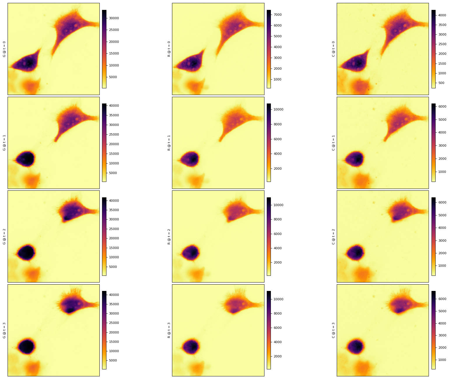
hv.opts.defaults(
hv.opts.Image(aspect=512 / 512),
hv.opts.Image("Cyan", cmap=plt.cm.Blues),
hv.opts.Image("Green", cmap=plt.cm.Greens),
hv.opts.Image("Red", cmap=plt.cm.Reds),
)
chans = (
hv.Image(dim.sel(C="C", Z=0)[0], group="cyan")
+ hv.Image(dim.sel(C="G", Z=0)[0], group="green")
+ hv.Image(dim.sel(C="R", Z=0)[0], group="red")
)
chans
nima.plot_img(dimm.sel(Z=0) - dim.sel(Z=0))
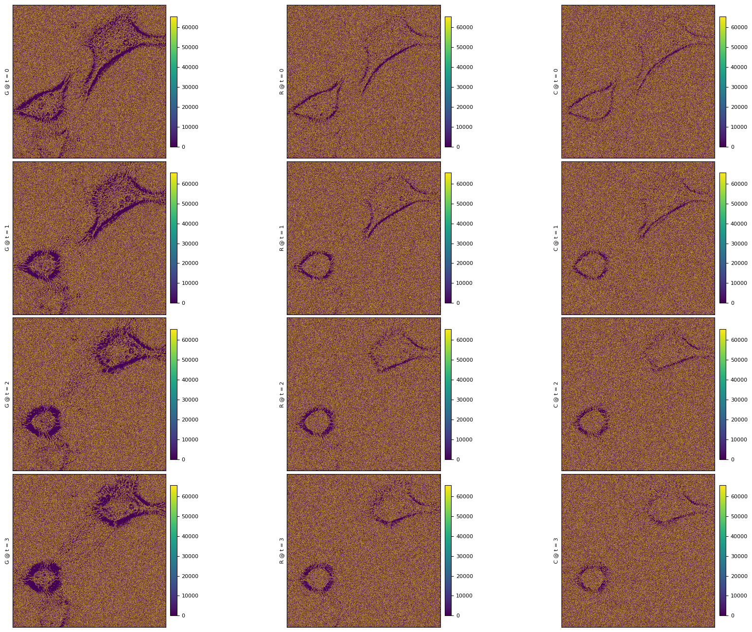
c = [(i, hv.Image(im)) for i, im in enumerate(dim.sel(C="C", Z=0))]
c = hv.HoloMap(c, kdims=["Frame"])
g = [(i, hv.Image(im)) for i, im in enumerate(dim.sel(C="G", Z=0))]
g = hv.HoloMap(g, kdims=["Frame"])
r = [(i, hv.Image(im)) for i, im in enumerate(dim.sel(C="R", Z=0))]
r = hv.HoloMap(r, kdims=["Frame"])
hv.output(holomap="auto")
hv.opts.defaults(hv.opts.Image(cmap="viridis"))
(c + g).select(Frame={0, 5, 6, 7, 10, 30}).cols(2)
c[::20].overlay("Frame")
wl = hv.Dimension("excitation wavelength", unit="nm")
c = c.add_dimension(wl, 1, 458)
g = g.add_dimension(wl, 1, 488)
r = r.add_dimension(wl, 1, 561)
channels = c.clone()
channels.update(g)
channels.update(r)
hv.opts.defaults(hv.opts.Image(cmap="viridis", frame_width=300, aspect="equal"))
channels[::5].grid(["Frame", "excitation wavelength"])
t = [(i, hv.Image(im)) for i, im in enumerate(dim.sel(C="C", Z=0))]
hv.HoloMap(
[(i, hv.Image(im)) for i, im in enumerate(dim.sel(C="C", Z=0))], kdims=["frame"]
)
[str(k) for k in dim.C.data]
['G', 'R', 'C']
hv.NdLayout(
{
k: hv.HoloMap(
[(i, hv.Image(im)) for i, im in enumerate(dim.sel(C=k, Z=0))],
kdims=["frame"],
)
for k in dim.C.data
},
kdims=["C"],
)[::4]
hv.opts.defaults(hv.opts.Image(cmap="viridis"), hv.opts.Image("A", aspect=2))
im = hv.Image(dim.sel(Z=0, C="G")[1])
im2 = hv.Image(dim.sel(Z=0, C="C")[1])
im3 = hv.Image(dimm.sel(Z=0, C="C")[1])
(
(im * hv.HLine(y=350 * 0.2))
+ im.sample(Y=350 * 0.2)
+ (im2 * hv.VLine(x=30))
+ im.sample(X=76) * im3.sample(X=30)
).cols(3)
On this page