2. Ratio Simulations#
%load_ext autoreload
%autoreload 2

import matplotlib.pyplot as plt
import numpy as np
import pandas as pd
import scipy
import skimage
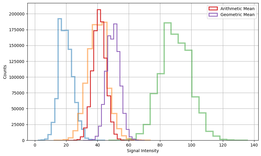
2.1. Poisson distribution for 3 channels#
This simulation compares the arithmetic and geometric averages of three signals, each following a Poisson distribution.
While the arithmetic average exhibits a slightly superior reduction in standard deviation, it’s noteworthy that the distribution of the arithmetic average tends to be more discernibly separated from the background when signals of different intensities are considered.
This insight lays the foundation for more robust segmentation methodologies tailored to multichannel images.
N = 1000000

rng = np.random.default_rng(1)

s1 = rng.poisson(20, N)
s2 = rng.poisson(40, N)
s3 = rng.poisson(90, N)

plt.figure(figsize=(10, 6))
plt.hist(s1, histtype="step", bins=20, lw=3, alpha=0.5)
plt.hist(s2, histtype="step", bins=20, lw=3, alpha=0.5)
plt.hist(s3, histtype="step", bins=20, lw=3, alpha=0.5)
plt.hist(
    np.power(s1 * s2 * s3, 1 / 3),
    histtype="step",
    bins=20,
    lw=2,
    label="Arithmetic Mean",
)
plt.hist(
    np.average([s1, s2, s3], axis=0),
    histtype="step",
    bins=20,
    lw=2,
    label="Geometric Mean",
)
plt.xlabel("Signal Intensity")
plt.ylabel("Counts")
plt.legend()
plt.grid()

# Compute standard deviations
s_avg_std = np.std(np.average([s1, s2, s3], axis=0))
s_cbrt_std = np.std(np.power(s1 * s2 * s3, 1 / 3))
# Print standard deviations
print(f"Standard Deviation of Arithmetic Mean of Signals: {s_avg_std:.3g}")
print(f"Standard Deviation of Geometric Mean of Signals: {s_cbrt_std:.3g}")
Standard Deviation of Arithmetic Mean of Signals: 4.08
Standard Deviation of Geometric Mean of Signals: 4.1
2.2. Ratio calculation#
We move on exploring the simulation of two channels (signals) and examining their ratios. Our goal is to understand how different averaging methods can influence the resulting distribution and statistical measures of these ratios. We’ll also introduce the concept of sliding window analysis to simulate image Gaussian filtering and explore its impact on the ratio calculation.
Let’s begin by generating two signals, “cyan” and “red,” each following a Poisson distribution with different intensities. We’ll plot histograms of their signal intensities to visualize their distributions.
# Set the number of pixels in the region of interest (ROI)
N = 999

# Generate Poisson-distributed signals for cyan and red channels
cyan = rng.poisson(50, N)
red = rng.poisson(50, N)

# Plot histograms of signal intensities
plt.figure(figsize=(10, 6))  # Set figure size
plt.hist(
    cyan, bins=30, histtype="step", lw=3, alpha=0.6, label="cyan", color="darkcyan"
)
plt.hist(red, bins=30, histtype="step", lw=3, alpha=0.6, label="red", color="indianred")
plt.xlabel("Signal Intensity")
plt.ylabel("Counts")
plt.title("Histograms of Signal Intensity")
plt.legend()
plt.grid()
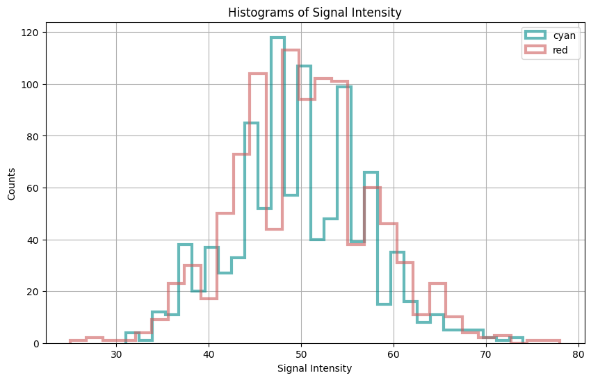
The histograms display the distribution of signal intensities for both the cyan and red channels.
Next, we’ll calculate the ratio between the cyan and red channels using various methods:
Simple Ratio: We’ll compute the ratio by dividing the cyan signal by the red signal.
Running Ratio Median: We’ll simulate image Mean filtering by applying a sliding window approach with a window size of 9 pixels over both channels and calculate the median of the ratios within each window.
Ratiorank Filter: This kind of filter employs a sliding window approach. Within each window, the ratiorank filter calculates the ratio between every possible pair of values from the cyan and red signal channels. For a window size of 9 pixels per channel, this results in a total of 81 unique ratio calculations. Finally, aggregating these ratios using the median provides a robust estimate of the ratio central tendency, capturing localized variations in signal ratios.
# 1. Calculate the ratio of cyan-over-red
ratio = cyan / red

# 2. Calculate the ratio after running average the signals
rr = np.convolve(cyan, np.ones(9) / 9, mode="valid") / np.convolve(
    red, np.ones(9) / 9, mode="valid"
)


# 3. Calculate the ratio using RatioRank
def rank(numerators, denominators):
    r = [num / den for num in numerators for den in denominators]
    return np.median(r)


def sliding_window(arr1, arr2, size=9):
    """Generate sliding window of size `size` over two input arrays `arr1` and `arr2`."""
    for i in range(len(arr1) - size + 1):
        yield arr1[i : i + size], arr2[i : i + size]


ratiorank = []
for window1, window2 in sliding_window(cyan, red):
    ratiorank.append(rank(window1, window2))

# Plot histogram of the ratio
plt.figure(figsize=(10, 6))
plt.hist(
    ratio,
    bins=30,
    histtype="step",
    lw=3,
    alpha=0.6,
    color="purple",
    label="Simple Ratio",
)
plt.hist(rr, bins=30, histtype="step", lw=2, alpha=0.6, label="Running Average")
plt.hist(
    ratiorank,
    bins=30,
    histtype="step",
    lw=2,
    alpha=0.6,
    color="blue",
    label="Median Ratiorank",
)

plt.xlabel("Cyan / Red Ratio")
plt.ylabel("Counts")
plt.title("Histogram of Cyan-over-Red Ratio")
plt.grid()
plt.legend()
plt.show()

# Plot probability plots for simple ratio, ratiorank, and running average
plt.figure(figsize=(10.5, 3.5))
# Simple ratio
plt.subplot(1, 3, 1)
scipy.stats.probplot(ratio, plot=plt, rvalue=True)
plt.title("Simple Ratio")
plt.xlabel("Theoretical Quantiles")
plt.ylabel("Ordered Values")
# Running average
plt.subplot(1, 3, 2)
scipy.stats.probplot(rr, plot=plt, rvalue=True)
plt.title("Running Average")
plt.xlabel("Theoretical Quantiles")
plt.ylabel("Ordered Values")
# Ratiorank
plt.subplot(1, 3, 3)
scipy.stats.probplot(ratiorank, plot=plt, rvalue=True)
plt.title("Ratiorank")
plt.xlabel("Theoretical Quantiles")
plt.ylabel("Ordered Values")
# Tight
plt.tight_layout()
plt.show()
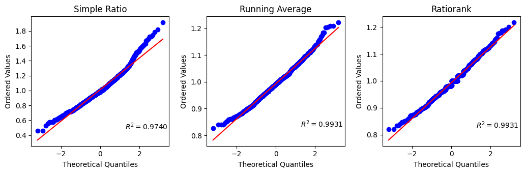
The simple ratio values exhibit a skewed distribution towards higher values, evident from the deviation observed in the probplot and the notable differences in the tails apparent in the q-q plot.
Indeed, ratiorank emerges as a promising alternative to both the simple ratio and running average methods in this context. By computing the median of 81 calculated ratios from sliding windows, ratiorank offers improved robustness and accuracy compared to the running average, which relies on fewer samples. This enhanced fidelity suggests ratiorank as a valuable approach for applications requiring precise ratio calculations,
Hence, the ratio of the entire ROI is accurately estimated from the median of the calculated distribution, as the mean may be unreliable for non-normally distributed data.
Additionally, signal averaging over the ROI prior to ratio calculation can be considered.
# 4. Calculate the ratio of averaged signals
ratio_of_avg = np.average(cyan) / np.average(red)
ratio_of_median = np.median(cyan) / np.median(red)

# Print statistical measures of the ratios
print(
    f"1. Simple Ratio (median vs. mean): {np.median(ratio):.3f} vs. {np.average(ratio):.3f}"
)
print(
    f"1. Running Ratio (median vs. mean): {np.median(rr):.3f} vs. {np.average(rr):.3f}"
)
print(
    f"1. Ratiorank (median vs. mean): {np.median(ratiorank):.3f} vs. {np.average(ratiorank):.3f}"
)
print(f"Ratio of (median vs.) Averages: ({ratio_of_median:.3f} vs.) {ratio_of_avg:.3f}")
1. Simple Ratio (median vs. mean): 1.000 vs. 1.014
1. Running Ratio (median vs. mean): 0.991 vs. 0.993
1. Ratiorank (median vs. mean): 0.983 vs. 0.993
Ratio of (median vs.) Averages: (1.000 vs.) 0.991
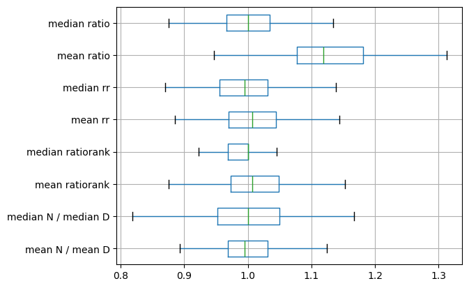
# Define variables
roi_size = 80
signal = 10
# Initialize lists to store results
ratios_med = []
ratios_avg = []
rrs_med = []
rrs_avg = []
rranks_med = []
rranks_avg = []
r_med = []
r_avg = []
# Perform simulation
for _ in range(199):
    # Generate random signals for cyan and red channels
    cyan = rng.poisson(signal, roi_size)
    red = rng.poisson(signal, roi_size)
    # Calculate simple ratios
    ratio = cyan / red
    # Calculate running averages
    rr = np.convolve(cyan, np.ones(9) / 9, mode="valid") / np.convolve(
        red, np.ones(9) / 9, mode="valid"
    )
    # Calculate ratiorank
    ratiorank = []
    for window1, window2 in sliding_window(cyan, red):
        ratiorank.append(rank(window1, window2))
    # Store results
    ratios_med.append(np.median(ratio))
    ratios_avg.append(np.mean(ratio))
    rrs_med.append(np.median(rr))
    rrs_avg.append(np.mean(rr))
    rranks_med.append(np.median(ratiorank))
    rranks_avg.append(np.mean(ratiorank))
    r_med.append(np.median(cyan) / np.median(red))
    r_avg.append(np.mean(cyan) / np.mean(red))

# Create DataFrame to organize results and plot boxplot
df = pd.DataFrame(
    np.column_stack((
        r_avg,
        r_med,
        rranks_avg,
        rranks_med,
        rrs_avg,
        rrs_med,
        ratios_avg,
        ratios_med,
    )),
    columns=[
        "mean N / mean D",
        "median N / median D",
        "mean ratiorank",
        "median ratiorank",
        "mean rr",
        "median rr",
        "mean ratio",
        "median ratio",
    ],
)
f = df.boxplot(vert=False, showfliers=False)
/tmp/ipykernel_2763/59477226.py:19: RuntimeWarning: divide by zero encountered in divide
  ratio = cyan / red
/tmp/ipykernel_2763/3370250907.py:12: RuntimeWarning: divide by zero encountered in scalar divide
  r = [num / den for num in numerators for den in denominators]
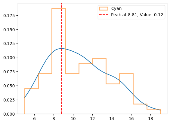
from scipy.stats import gaussian_kde

# Evaluate the KDE on a grid of points
x_grid = np.linspace(cyan.min(), cyan.max(), 1000)
y_kde = gaussian_kde(cyan)(x_grid)  # Evaluate the KDE at x_grid points

# Plot the KDE smoothed line
plt.plot(x_grid, y_kde)

plt.hist(cyan, density=1, bins=10, histtype="step", lw=2, alpha=0.6, label="Cyan")

# Find the peak position of the KDE
peak_position = x_grid[np.argmax(y_kde)]
peak_value = np.max(y_kde)

# Plot the peak position
plt.axvline(
    x=peak_position,
    color="r",
    linestyle="--",
    label=f"Peak at {peak_position:.2f}, Value: {peak_value:.2f}",
)
plt.legend()
plt.show()
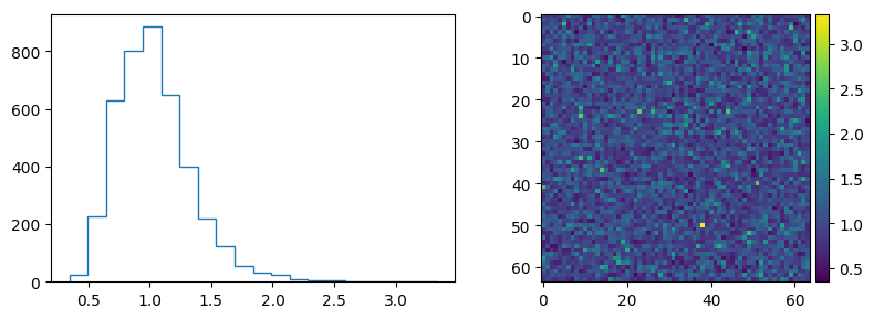
As an image.
TODO: Complete with Running-ratio and Ratiorank.
im_cyan = skimage.util.random_noise(25 * np.ones([64, 64]), mode="poisson", clip=0)
im_red = skimage.util.random_noise(25 * np.ones([64, 64]), mode="poisson", clip=0)
im_ratio = im_cyan / im_red

plt.figure(figsize=(8, 3))
plt.subplot(1, 2, 2)
skimage.io.imshow(im_ratio)
plt.subplot(1, 2, 1)
plt.hist(im_ratio.ravel(), histtype="step", bins=20)
plt.show()
/tmp/ipykernel_2763/2274224295.py:7: FutureWarning: `imshow` is deprecated since version 0.25 and will be removed in version 0.27. Please use `matplotlib`, `napari`, etc. to visualize images.
  skimage.io.imshow(im_ratio)
/home/runner/work/nima/nima/.venv/lib/python3.14/site-packages/skimage/io/_plugins/matplotlib_plugin.py:158: UserWarning: Float image out of standard range; displaying image with stretched contrast.
  lo, hi, cmap = _get_display_range(image)
2.3. MAYBE/TODO:#
simulare fret e bt:
$S^{561} = R$
$S^{488} = G (1 - E) + R (\alpha + E)$
$S^{458} = C (1 - E) + R (\beta + E)$
test ch1, ch2, ch3 and geometric average
test cross-correlation
consider detector gain in simulated error
simulate 3D obj + PSF in generation of synthetic data
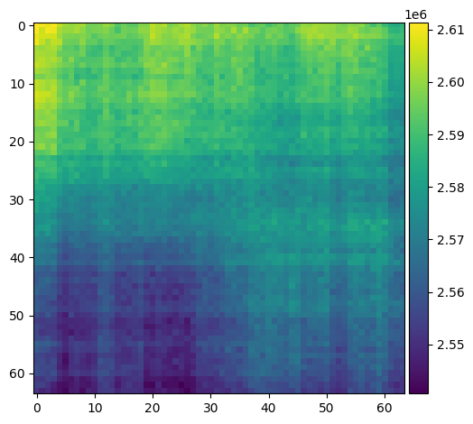
from scipy.ndimage import correlate as ic

skimage.io.imshow(ic(im_cyan, im_red))
/tmp/ipykernel_2763/3093962468.py:3: FutureWarning: `imshow` is deprecated since version 0.25 and will be removed in version 0.27. Please use `matplotlib`, `napari`, etc. to visualize images.
  skimage.io.imshow(ic(im_cyan, im_red))
/home/runner/work/nima/nima/.venv/lib/python3.14/site-packages/skimage/io/_plugins/matplotlib_plugin.py:158: UserWarning: Float image out of standard range; displaying image with stretched contrast.
  lo, hi, cmap = _get_display_range(image)
<matplotlib.image.AxesImage at 0x7fc0bed8a5d0>