1. Levenberg Marquardt Fitting#
1.1. Conventions#
S0 Signal for unbound state
S1 Signal for bound state
K equilibrium constant (Kd or pKa)
order data from unbound to bound (e.g. cl: 0–>150 mM; pH 9–>5)
import contextlib
import multiprocessing as mp
import os

if mp.get_start_method(allow_none=True) != "fork":
    with contextlib.suppress(RuntimeError, ValueError):
        mp.set_start_method("fork", force=True)

import warnings

import arviz as az
import corner
import lmfit
import matplotlib.pyplot as plt
import numpy as np
import pandas as pd
import pymc as pm
import scipy
import seaborn as sb

from clophfit.fitting.core import (
    DataArray,
    Dataset,
    fit_binding_glob,
    weight_multi_ds_titration,
)
from clophfit.fitting.plotting import plot_emcee, print_emcee

warnings.filterwarnings(
    "ignore",
    message=r"AffineScalarFunc\.error_components\(\) is currently an instance method\.",
    category=FutureWarning,
    module=r"uncertainties\.core",
)
warnings.filterwarnings(
    "ignore",
    message=r"AffineScalarFunc\.derivatives\(\) is deprecated\.",
    category=FutureWarning,
    module=r"uncertainties\.core",
)


%load_ext autoreload
%autoreload 2
1.2. Single Cl titration.#
df = pd.read_table("../../tests/data/copyIP.txt")
df["F"] /= np.max(df["F"])
sb.scatterplot(data=df, x="cl", y="F", hue=df.cl, palette="crest", s=200)
<Axes: xlabel='cl', ylabel='F'>
In general we can use either lmfit.minimize() -> res or lmfit.Minimizer -> mini.
def fz(x, S0, S1, Kd):
return (S0 + S1 * x / Kd) / (1 + x / Kd)
def residual(pars, x, y=None):
S0 = pars["S0"]
S1 = pars["S1"]
Kd = pars["Kd"]
model = fz(x, S0, S1, Kd)
if y is None:
return model
return np.array(y - model)
params = lmfit.Parameters()
params.add("S0", value=df.F[0], min=0, max=2)
params.add("S1", value=100, min=-0.1, max=2)
params.add("Kd", value=50, min=0, max=200)
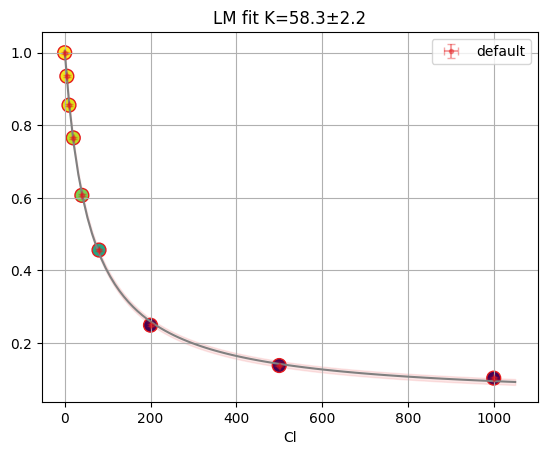
res = lmfit.minimize(residual, params, args=(df.cl, df.F))
xdelta = (df.cl.max() - df.cl.min()) / 500
xfit = np.arange(df.cl.min() - xdelta, df.cl.max() + xdelta, xdelta)
yfit = residual(res.params, xfit)
print(lmfit.fit_report(res.params))
plt.plot(df.cl, df.F, "o", xfit, yfit, "-")
[[Variables]]
    S0:  1.00381551 +/- 0.00652315 (0.65%) (init = 1)
    S1:  0.04204737 +/- 0.00478495 (11.38%) (init = 2)
    Kd:  58.3187768 +/- 2.24602959 (3.85%) (init = 50)
[[Correlations]] (unreported correlations are < 0.100)
    C(S1, Kd) = -0.7123
    C(S0, Kd) = -0.6562
    C(S0, S1) = +0.2747
[<matplotlib.lines.Line2D at 0x7ff2363aeba0>,
 <matplotlib.lines.Line2D at 0x7ff2363aecf0>]
mini = lmfit.Minimizer(residual, params, fcn_args=(df.cl, df.F))
res = mini.minimize()
ci, tr = lmfit.conf_interval(mini, res, sigmas=[0.68, 0.95], trace=True)
print(lmfit.ci_report(ci, with_offset=False, ndigits=2))
print(lmfit.fit_report(res, show_correl=False, sort_pars=True))
    95.00% 68.00% _BEST_ 68.00% 95.00%
 S0:   0.99   1.00   1.00   1.01   1.02
 S1:   0.02   0.03   0.04   0.05   0.06
 Kd:  53.13  55.95  58.32  60.79  64.07
[[Fit Statistics]]
    # fitting method   = leastsq
    # function evals   = 43
    # data points      = 9
    # variables        = 3
    chi-square         = 4.6992e-04
    reduced chi-square = 7.8320e-05
    Akaike info crit   = -82.7415766
    Bayesian info crit = -82.1499028
[[Variables]]
    Kd:  58.3187768 +/- 2.24602959 (3.85%) (init = 50)
    S0:  1.00381551 +/- 0.00652315 (0.65%) (init = 1)
    S1:  0.04204737 +/- 0.00478495 (11.38%) (init = 2)
mini.params.add("__lnsigma", value=np.log(0.1), min=np.log(0.001), max=np.log(2))
emcee_res = mini.emcee(
    nwalkers=int(os.environ.get("CLOPHFIT_DOCS_EMCEE_NWALKERS", "40")),
    workers=int(os.environ.get("CLOPHFIT_EMCEE_WORKERS", "1")),
    is_weighted=False,
    thin=int(os.environ.get("CLOPHFIT_DOCS_EMCEE_THIN", "40")),
    burn=int(os.environ.get("CLOPHFIT_DOCS_EMCEE_BURN", "150")),
    steps=int(os.environ.get("CLOPHFIT_DOCS_EMCEE_STEPS", "1800")),
    progress=False,
)
The chain is shorter than 50 times the integrated autocorrelation time for 4 parameter(s). Use this estimate with caution and run a longer chain!
N/50 = 6;
tau: [17.79940462 21.68732086 20.96742581 41.1081538 ]
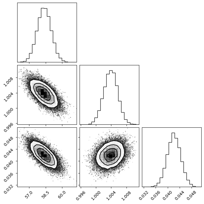
fig = plt.figure(figsize=(7, 7))
f = corner.corner(emcee_res.flatchain.to_numpy(), fig=fig)
# Extract parameter values and standard errors from lmfit result
S0_mu = res.params["S0"].value
S1_mu = res.params["S1"].value
Kd_mu = res.params["Kd"].value
S0_std = res.params["S0"].stderr
S1_std = res.params["S1"].stderr
Kd_std = res.params["Kd"].stderr

cov_matrix = res.covar

# Define PyMC3 model
with pm.Model() as model:
    # Define multivariate normal priors for parameters
    pars = pm.MvNormal("pars", mu=[S0_mu, S1_mu, Kd_mu], cov=cov_matrix, shape=3)
    S0 = pars[0]
    S1 = pars[1]
    Kd = pars[2]

    y_pred = pm.Deterministic("y_pred", fz(df.cl.to_numpy(), S0, S1, Kd))
    # Define likelihood
    likelihood = pm.Normal("likelihood", mu=y_pred, sigma=1, observed=df.F.to_numpy())
    # Run the inference
    trace = pm.sample(
        2000,
        tune=1000,
        cores=int(os.environ.get("CLOPHFIT_DOCS_PYMC_CORES", "1")),
        progressbar=False,
        mp_ctx=mp.get_context("fork"),
    )
Initializing NUTS using jitter+adapt_diag...
Sequential sampling (2 chains in 1 job)
NUTS: [pars]
Sampling 2 chains for 1_000 tune and 2_000 draw iterations (2_000 + 4_000 draws total) took 5 seconds.
We recommend running at least 4 chains for robust computation of convergence diagnostics
az.plot_dist(trace, var_names=["pars"], ci_prob=0.95, point_estimate="median")
<arviz_plots.plot_collection.PlotCollection at 0x7ff2284516a0>
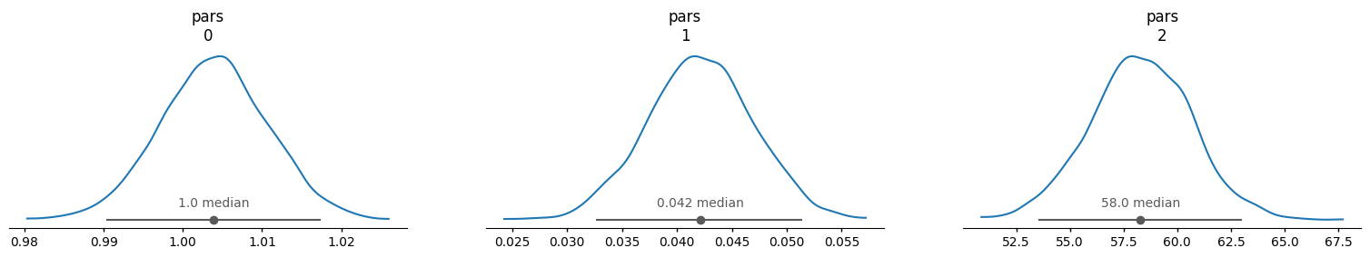
pm.stats.summary(trace)
| mean | sd | eti89_lb | eti89_ub | ess_bulk | ess_tail | r_hat | mcse_mean | mcse_sd | |
|---|---|---|---|---|---|---|---|---|---|
| pars[0] | 1.0039 | 0.0068 | 0.99 | 1 | 1708 | 1956 | 1.00 | 0.00016 | 0.00012 |
| pars[1] | 0.0421 | 0.0048 | 0.034 | 0.05 | 1571 | 1608 | 1.00 | 0.00012 | 8.5e-05 |
| pars[2] | 58.3 | 2.35 | 54 | 62 | 1427 | 1565 | 1.00 | 0.062 | 0.044 |
| y_pred[0] | 1.0039 | 0.0068 | 0.99 | 1 | 1708 | 1956 | 1.00 | 0.00016 | 0.00012 |
| y_pred[1] | 0.9278 | 0.0048 | 0.92 | 0.94 | 2259 | 2586 | 1.00 | 0.0001 | 7.1e-05 |
| y_pred[2] | 0.8629 | 0.0041 | 0.86 | 0.87 | 3065 | 2975 | 1.00 | 7.4e-05 | 5.2e-05 |
| y_pred[3] | 0.758 | 0.0046 | 0.75 | 0.77 | 2632 | 2984 | 1.00 | 9.1e-05 | 6.3e-05 |
| y_pred[4] | 0.6123 | 0.0059 | 0.6 | 0.62 | 2020 | 2145 | 1.00 | 0.00013 | 9.4e-05 |
| y_pred[5] | 0.4474 | 0.0059 | 0.44 | 0.46 | 1907 | 2249 | 1.00 | 0.00014 | 9.7e-05 |
| y_pred[6] | 0.2591 | 0.0039 | 0.25 | 0.27 | 2430 | 2565 | 1.00 | 7.9e-05 | 5.5e-05 |
| y_pred[7] | 0.1425 | 0.00282 | 0.14 | 0.15 | 2835 | 2768 | 1.00 | 5.3e-05 | 3.7e-05 |
| y_pred[8] | 0.0951 | 0.0034 | 0.09 | 0.1 | 1958 | 2155 | 1.00 | 7.7e-05 | 5.3e-05 |
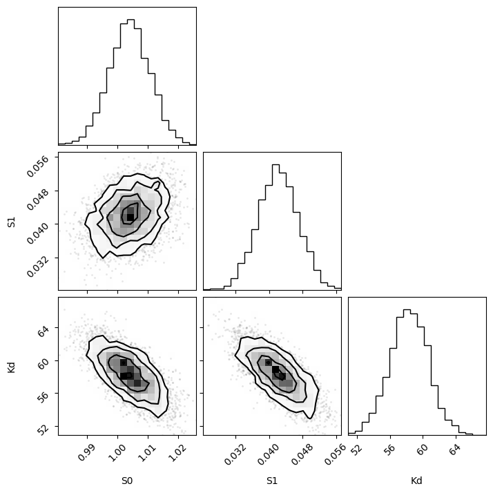
# Extract pars samples for corner plot
pars_samples = trace.posterior["pars"].to_numpy().reshape(-1, 3)
f = corner.corner(pars_samples, labels=["S0", "S1", "Kd"])
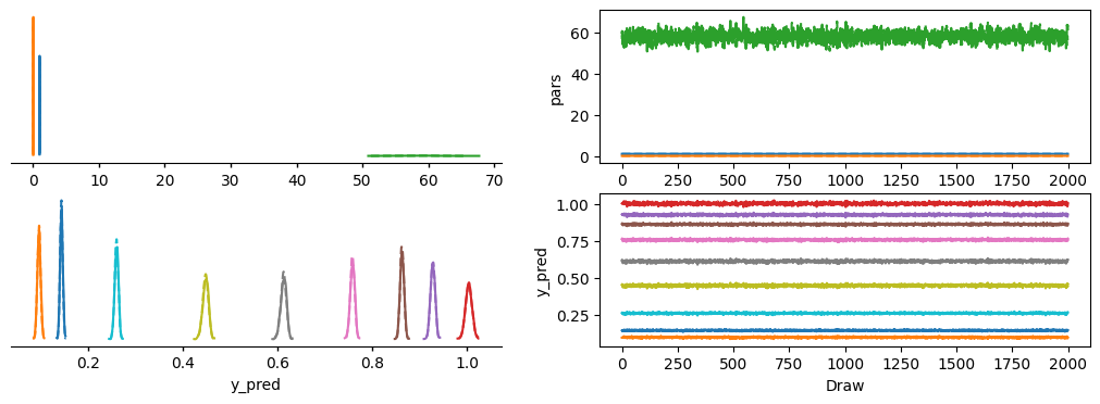
az.plot_trace_dist(trace)
<arviz_plots.plot_collection.PlotCollection at 0x7ff2280b4410>
def plot_scatter_matrix(res, tr):
names = res.params.keys()
gs = plt.GridSpec(4, 4)
sx = {}
sy = {}
for i, fixed in enumerate(names):
for j, free in enumerate(names):
sharex = sx.get(j)
sharey = sy.get(i)
ax = plt.subplot(gs[i, j], sharex=sharex, sharey=sharey)
if sharex is None:
sx[j] = ax
if sharey is None:
sy[i] = ax
if i < 3:
plt.setp(ax.get_xticklabels(), visible=True)
else:
ax.set_xlabel(free)
if j > 0:
plt.setp(ax.get_yticklabels(), visible=False)
else:
ax.set_ylabel(fixed)
rest = tr[fixed]
prob = rest["prob"]
f = prob < 0.96
x, y = rest[free], rest[fixed]
ax.scatter(x[f], y[f], c=1 - prob[f], s=25 * (1 - prob[f] + 0.5))
ax.autoscale(1, 1)
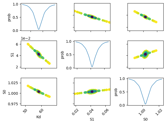
plot_scatter_matrix(res, tr)
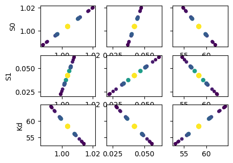
The plots shown below, akin to the examples provided in lmfit documentation, are computationally intensive. They operate under the assumption of a parabolic parameter space. However, it’s worth noting that these plots provide similar information to that yielded by a Monte Carlo simulation.
def plot_conf_interval_matrix(res, tr):
    names = list(res.params.keys())
    plt.figure()

    for i in range(3):
        for j in range(3):
            idx = 9 - j * 3 - i
            ax = plt.subplot(3, 3, idx)
            ax.ticklabel_format(style="sci", scilimits=(-2, 2), axis="y")

            # Set-up labels and tick marks
            ax.tick_params(labelleft=False, labelbottom=False)
            if idx in {1, 4, 7}:
                plt.ylabel(names[j])
                ax.tick_params(labelleft=True)
            if idx == 1:
                ax.tick_params(labelleft=True)
            if idx in {7, 8, 9}:
                plt.xlabel(names[i])
                ax.tick_params(labelbottom=True)
                [label.set_rotation(45) for label in ax.get_xticklabels()]

            if i != j:
                x, y, m = lmfit.conf_interval2d(mini, res, names[i], names[j], 20, 20)
                plt.contourf(x, y, m, np.linspace(0, 1, 10))

                x = tr[names[i]][names[i]]
                y = tr[names[i]][names[j]]
                pr = tr[names[i]]["prob"]
                s = np.argsort(x)
                plt.scatter(x[s], y[s], c=pr[s], s=30, lw=1)

            else:
                x = tr[names[i]][names[i]]
                y = tr[names[i]]["prob"]

                t, s = np.unique(x, return_index=True)
                f = scipy.interpolate.interp1d(t, y[s], "slinear")
                xn = np.linspace(x.min(), x.max(), 50)
                plt.plot(xn, f(xn), lw=1)
                plt.ylabel("prob")
                ax.tick_params(labelleft=True)

    plt.tight_layout()


plot_conf_interval_matrix(res, tr)
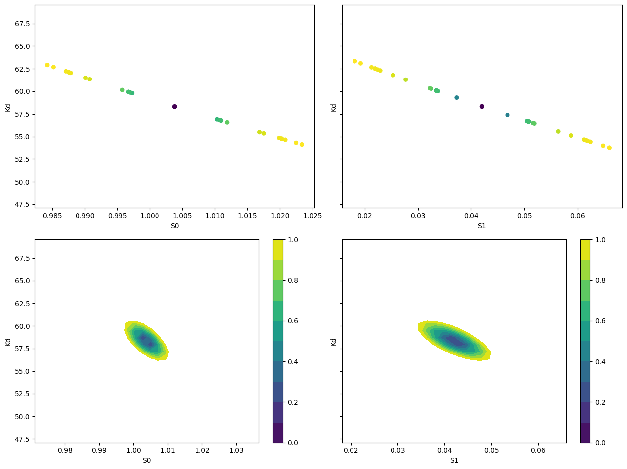
def plot_conf_intervals(mini, res):
    # Report fit parameters
    lmfit.report_fit(res.params, min_correl=0.25)

    # Calculate confidence intervals and traces
    ci, trace = lmfit.conf_interval(mini, res, sigmas=[1, 2], trace=True)
    lmfit.printfuncs.report_ci(ci)

    # Create subplots
    _fig, axes = plt.subplots(2, 2, figsize=(12.8, 9.6), sharey=True)

    # Plot scatter plots for S0 and S1
    plot_scatter_trace(axes[0][0], trace["S0"], "S0", "Kd")
    plot_scatter_trace(axes[0][1], trace["S1"], "S1", "Kd")

    # Plot 2D confidence intervals for S0 and S1
    plot_2d_conf_interval(axes[1][0], mini, res, "S0", "Kd")
    plot_2d_conf_interval(axes[1][1], mini, res, "S1", "Kd")

    plt.tight_layout()


def plot_scatter_trace(ax, trace_data, xlabel, ylabel):
    cx, cy, prob = trace_data[xlabel], trace_data[ylabel], trace_data["prob"]
    ax.scatter(cx, cy, c=prob, s=30)
    ax.set_xlabel(xlabel)
    ax.set_ylabel(ylabel)


def plot_2d_conf_interval(ax, mini, res, xparam, yparam):
    # Calculate 2D confidence interval
    cx, cy, grid = lmfit.conf_interval2d(mini, res, xparam, yparam, 30, 30)
    # Plot the contourf with a colorbar
    ctp = ax.contourf(cx, cy, grid, np.linspace(0, 1, 11))
    fig = ax.figure
    fig.colorbar(ctp, ax=ax)
    ax.set_xlabel(xparam)
    ax.set_ylabel(yparam)


plot_conf_intervals(mini, res)
[[Variables]]
    S0:  1.00381551 +/- 0.00652315 (0.65%) (init = 1)
    S1:  0.04204737 +/- 0.00478495 (11.38%) (init = 2)
    Kd:  58.3187768 +/- 2.24602959 (3.85%) (init = 50)
[[Correlations]] (unreported correlations are < 0.250)
    C(S1, Kd) = -0.7123
    C(S0, Kd) = -0.6562
    C(S0, S1) = +0.2747
       95.45%    68.27%    _BEST_    68.27%    95.45%
 S0:  -0.01626  -0.00708   1.00382  +0.00712  +0.01647
 S1:  -0.02009  -0.00857   0.04205  +0.00875  +0.01988
 Kd:  -5.32871  -2.37867  58.31878  +2.49056  +5.92497
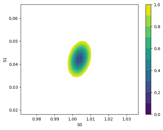
f, ax = plt.subplots(1, 1)
plot_2d_conf_interval(ax, mini, res, "S0", "S1")
1.2.1. Using clophfit.fitting#
da = DataArray(df["cl"].to_numpy(), df["F"].to_numpy())
ds = Dataset.from_da(da)
weight_multi_ds_titration(ds)
f_res = fit_binding_glob(ds)

f_res.figure
emcee_res = f_res.mini.emcee(
    steps=3000, burn=300, workers=4, nwalkers=30, seed=1, progress=False
)
plot_emcee(emcee_res.flatchain)
print_emcee(emcee_res)
The chain is shorter than 50 times the integrated autocorrelation time for 3 parameter(s). Use this estimate with caution and run a longer chain!
N/50 = 60;
tau: [98.06551952 63.16598997 97.66342074]

Maximum Likelihood Estimation from emcee
-------------------------------------------------
Parameter   MLE Value Median Value Uncertainty
K        58.31879    58.34677     0.63780
S0_default     1.00380     1.00383     0.00184
S1_default     0.04217     0.04205     0.00227

Error estimates from emcee:
------------------------------------------------------
Parameter  -2sigma  -1sigma   median  +1sigma  +2sigma
  K        57.0693  57.7129  58.3468  58.9888  59.5966
  S0_default     1.0001   1.0019   1.0038   1.0056   1.0073
  S1_default     0.0375   0.0398   0.0420   0.0443   0.0465

Maximum Likelihood Estimation (MLE):
----------------------------------
K: 58.319
S0_default: 1.004
S1_default: 0.042


1 sigma spread = 0.638
2 sigma spread = 1.290
emcee_res.flatchain.describe()
| K | S0_default | S1_default | |
|---|---|---|---|
| count | 81000.000000 | 81000.000000 | 81000.000000 |
| mean | 58.350361 | 1.003804 | 0.042065 |
| std | 0.642355 | 0.001846 | 0.002271 |
| min | 55.897535 | 0.995657 | 0.031368 |
| 25% | 57.915808 | 1.002570 | 0.040534 |
| 50% | 58.346770 | 1.003830 | 0.042049 |
| 75% | 58.779289 | 1.005055 | 0.043581 |
| max | 61.319147 | 1.011291 | 0.051221 |
1.3. Fit titration with multiple datasets#
For example data collected with multiple labelblocks in Tecan plate reader.
“A01”: pH titration with y1 and y2.
df = pd.read_csv("../../tests/data/A01.dat", sep=" ", names=["x", "1", "2"])
df = df[::-1].reset_index(drop=True)
df
| x | 1 | 2 | |
|---|---|---|---|
| 0 | 9.030000 | 29657.0 | 22885.0 |
| 1 | 8.373333 | 35200.0 | 16930.0 |
| 2 | 7.750000 | 44901.0 | 9218.0 |
| 3 | 7.073333 | 53063.0 | 3758.0 |
| 4 | 6.460000 | 54202.0 | 2101.0 |
| 5 | 5.813333 | 54851.0 | 1542.0 |
| 6 | 4.996667 | 51205.0 | 1358.0 |
1.3.1. lmfit of single y1 using analytical Jacobian#
It computes the Jacobian of the fz. Mind that the residual (i.e. y - fz) will be actually minimized.
import sympy

x, S0_1, S1_1, K = sympy.symbols("x S0_1 S1_1 K")
f = (S0_1 + S1_1 * 10 ** (K - x)) / (1 + 10 ** (K - x))
print(sympy.diff(f, S0_1))
print(sympy.diff(f, S1_1))
print(sympy.diff(f, K))
1/(10**(K - x) + 1)
10**(K - x)/(10**(K - x) + 1)
10**(K - x)*S1_1*log(10)/(10**(K - x) + 1) - 10**(K - x)*(10**(K - x)*S1_1 + S0_1)*log(10)/(10**(K - x) + 1)**2
x, S0, S1, K = sympy.symbols("x S0 S1 K")
f = S0 + (S1 - S0) * x / K / (1 + x / K)
sympy.diff(f, S0)
sympy.diff(f, S1)
sympy.diff(f, K)
# if is_ph:
f = S0 + (S1 - S0) * 10 ** (K - x) / (1 + 10 ** (K - x))
sympy.diff(f, S0)
sympy.diff(f, S1)
sympy.diff(f, K)
def residual(pars, x, data):
    S0 = pars["S0"]
    S1 = pars["S1"]
    K = pars["K"]
    # model = (S0 + S1 * x / Kd) / (1 + x / Kd)
    x = np.array(x)
    y = np.array(data)
    model = (S0 + S1 * 10 ** (K - x)) / (1 + 10 ** (K - x))
    if data is None:
        return model
    return np.array(y - model)


# Try Jacobian
def dfunc(pars, x, data=None):
    S0_1 = pars["S0"]
    S1_1 = pars["S1"]
    K = pars["K"]
    kx = np.array(10 ** (K - x))
    return np.array([
        -1 / (kx + 1),
        -kx / (kx + 1),
        -kx * np.log(10) * (S1_1 / (kx + 1) - (kx * S1_1 + S0_1) / (kx + 1) ** 2),
    ])


params = lmfit.Parameters()
params.add("S0", value=25000)
params.add("S1", value=50000, min=0.0)
params.add("K", value=7, min=2.0, max=12.0)

mini = lmfit.Minimizer(residual, params, fcn_args=(df.x,), fcn_kws={"data": df["1"]})
res = mini.leastsq(Dfun=dfunc, col_deriv=True, ftol=1e-8)
print(lmfit.report_fit(res))
ci = lmfit.conf_interval(mini, res, sigmas=[1, 2, 3])
[[Fit Statistics]]
    # fitting method   = leastsq
    # function evals   = 9
    # data points      = 7
    # variables        = 3
    chi-square         = 12308015.2
    reduced chi-square = 3077003.79
    Akaike info crit   = 106.658958
    Bayesian info crit = 106.496688
[[Variables]]
    S0:  26638.8377 +/- 2455.91825 (9.22%) (init = 25000)
    S1:  54043.3592 +/- 979.995977 (1.81%) (init = 50000)
    K:   8.06961091 +/- 0.14940678 (1.85%) (init = 7)
[[Correlations]] (unreported correlations are < 0.100)
    C(S0, K)  = -0.7750
    C(S1, K)  = -0.4552
    C(S0, S1) = +0.2046
None
print(lmfit.ci_report(ci, with_offset=False, ndigits=2))
    99.73% 95.45% 68.27% _BEST_ 68.27% 95.45% 99.73%
 S0:-58596.9018262.4323743.2826638.8429197.6132638.1538999.44
 S1:47850.5551309.0552945.1454043.3655156.5456872.9060768.74
 K :   7.09   7.67   7.91   8.07   8.23   8.50   9.58
1.3.2. using lmfit with np.r_ trick#
def residual2(pars, x, data=None):
    K = pars["K"]
    S0_1 = pars["S0_1"]
    S1_1 = pars["S1_1"]
    S0_2 = pars["S0_2"]
    S1_2 = pars["S1_2"]
    model_0 = (S0_1 + S1_1 * 10 ** (K - x[0])) / (1 + 10 ** (K - x[0]))
    model_1 = (S0_2 + S1_2 * 10 ** (K - x[1])) / (1 + 10 ** (K - x[1]))
    if data is None:
        return np.r_[model_0, model_1]
    return np.r_[data[0] - model_0, data[1] - model_1]


params2 = lmfit.Parameters()
params2.add("K", value=7.0, min=2.0, max=12.0)
params2.add("S0_1", value=df["1"][0], min=0.0)
params2.add("S0_2", value=df["2"][0], min=0.0)
params2.add("S1_1", value=df["1"].iloc[-1], min=0.0)
params2.add("S1_2", value=df["2"].iloc[-1], min=0.0)
mini2 = lmfit.Minimizer(
    residual2, params2, fcn_args=([df.x, df.x],), fcn_kws={"data": [df["1"], df["2"]]}
)
res2 = mini2.minimize()
print(lmfit.fit_report(res2))

ci2, tr2 = lmfit.conf_interval(mini2, res2, sigmas=[0.68, 0.95], trace=True)
print(lmfit.ci_report(ci2, with_offset=False, ndigits=2))
[[Fit Statistics]]
    # fitting method   = leastsq
    # function evals   = 37
    # data points      = 14
    # variables        = 5
    chi-square         = 12471473.3
    reduced chi-square = 1385719.25
    Akaike info crit   = 201.798560
    Bayesian info crit = 204.993846
[[Variables]]
    K:     8.07255029 +/- 0.07600777 (0.94%) (init = 7)
    S0_1:  26601.3458 +/- 1425.69913 (5.36%) (init = 29657)
    S0_2:  25084.4189 +/- 1337.07982 (5.33%) (init = 22885)
    S1_1:  54034.5806 +/- 627.642479 (1.16%) (init = 51205)
    S1_2:  1473.57871 +/- 616.944649 (41.87%) (init = 1358)
[[Correlations]] (unreported correlations are < 0.100)
    C(K, S0_1)    = -0.6816
    C(K, S0_2)    = +0.6255
    C(S0_1, S0_2) = -0.4264
    C(K, S1_1)    = -0.3611
    C(K, S1_2)    = +0.3161
    C(S0_2, S1_1) = -0.2259
    C(S0_1, S1_2) = -0.2155
    C(S1_1, S1_2) = -0.1141
      95.00% 68.00% _BEST_ 68.00% 95.00%
 K   :   7.91   7.99   8.07   8.15   8.24
 S0_1:23210.9025078.6226601.3528045.4929623.53
 S0_2:22232.9723723.9425084.4226514.8828263.75
 S1_1:52629.0453378.2454034.5854695.2655460.17
 S1_2:  72.04 824.011473.582118.982855.89
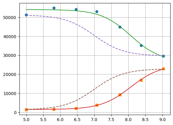
xfit = np.linspace(df.x.min(), df.x.max(), 100)
yfit0 = residual2(params2, [xfit, xfit])
yfit0 = yfit0.reshape(2, 100)
yfit = residual2(res2.params, [xfit, xfit])
yfit = yfit.reshape(2, 100)
plt.plot(df.x, df["1"], "o", df.x, df["2"], "s")
plt.plot(xfit, yfit[0], "-", xfit, yfit[1], "-")
plt.plot(xfit, yfit0[0], "--", xfit, yfit0[1], "--")
plt.grid(visible=True)
1.3.3. lmfit constraints aiming for generality#
I believe a name convention would be more robust than relying on OrderedDict Params object.
["S0", "1"][0]
'S0'
def exception_fcn_handler(func):
    def inner_function(*args, **kwargs):
        try:
            return func(*args, **kwargs)
        except TypeError:
            print(
                f"{func.__name__} only takes (1D) vector as argument besides lmfit.Parameters."
            )

    return inner_function


@exception_fcn_handler
def titration_pH(params, pH):
    p = {k.split("_")[0]: v for k, v in params.items()}
    return (p["S0"] + p["S1"] * 10 ** (p["K"] - pH)) / (1 + 10 ** (p["K"] - pH))


def residues(params, x, y, fcn):
    return y - fcn(params, x)


p1 = lmfit.Parameters()
p2 = lmfit.Parameters()
p1.add("K_1", value=7.0, min=2.0, max=12.0)
p2.add("K_2", value=7.0, min=2.0, max=12.0)
p1.add("S0_1", value=df["1"].iloc[0], min=0.0)
p2.add("S0_2", value=df["2"].iloc[0], min=0.0)
p1.add("S1_1", value=df["1"].iloc[-1], min=0.0)
p2.add("S1_2", value=df["2"].iloc[-1])

print(
    residues(p1, np.array(df.x), [1.97, 1.8, 1.7, 0.1, 0.1, 0.16, 0.01], titration_pH)
)


def gobjective(params, xl, yl, fcnl):
    nset = len(xl)
    res = []
    for i in range(nset):
        pi = {k: v for k, v in params.valuesdict().items() if k[-1] == f"{i + 1}"}
        res = np.r_[res, residues(pi, xl[i], yl[i], fcnl[i])]
        # res = np.r_[res, yl[i] - fcnl[i](parsl[i], x[i])]
    return res


print(
    gobjective(p1 + p2, [df.x, df.x], [df["1"], df["2"]], [titration_pH, titration_pH])
)
[-29854.26823732 -30530.32007939 -32908.60749879 -39523.42660007
 -46381.47878947 -49888.5091843  -50993.25866394]
[  -199.23823732   4667.87992061  11990.69250121  13539.47339993
   7820.42121053   4962.3308157     211.73133606    199.04406603
  -5080.73278499 -10416.86307191  -9270.08900503  -4075.72045662
  -1131.04796128   -211.52498939]
Here single.
mini = lmfit.Minimizer(
residues,
p1,
fcn_args=(
df.x,
df["1"],
titration_pH,
),
)
res = mini.minimize()
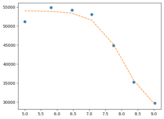
fit = titration_pH(res.params, df.x)
print(lmfit.report_fit(res))
plt.plot(df.x, df["1"], "o", df.x, fit, "--")
ci = lmfit.conf_interval(mini, res, sigmas=[1, 2])
lmfit.printfuncs.report_ci(ci)
[[Fit Statistics]]
    # fitting method   = leastsq
    # function evals   = 25
    # data points      = 7
    # variables        = 3
    chi-square         = 12308015.2
    reduced chi-square = 3077003.79
    Akaike info crit   = 106.658958
    Bayesian info crit = 106.496688
[[Variables]]
    K_1:   8.06961042 +/- 0.14940740 (1.85%) (init = 7)
    S0_1:  26638.8440 +/- 2455.92762 (9.22%) (init = 29657)
    S1_1:  54043.3607 +/- 979.995185 (1.81%) (init = 51205)
[[Correlations]] (unreported correlations are < 0.100)
    C(K_1, S0_1)  = -0.7750
    C(K_1, S1_1)  = -0.4552
    C(S0_1, S1_1) = +0.2046
None
         95.45%    68.27%    _BEST_    68.27%    95.45%
 K_1 :  -0.40197  -0.15948   8.06961  +0.16276  +0.42592
 S0_1:-8376.39586-2895.5681226638.84401+2558.76794+5999.32366
 S1_1:-2734.30835-1098.2218354043.36069+1113.18102+2829.55353
Now global.
pg = p1 + p2
pg["K_2"].expr = "K_1"
gmini = lmfit.Minimizer(
gobjective,
pg,
fcn_args=([df.x[:], df.x], [df["1"][:], df["2"]], [titration_pH, titration_pH]),
)
gres = gmini.minimize()
print(lmfit.fit_report(gres))
pp1 = {k: v for k, v in gres.params.valuesdict().items() if k.split("_")[1] == f"{1}"}
pp2 = {k: v for k, v in gres.params.valuesdict().items() if k.split("_")[1] == f"{2}"}
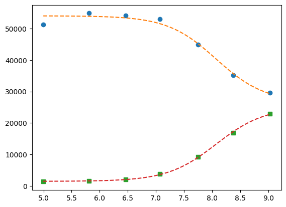
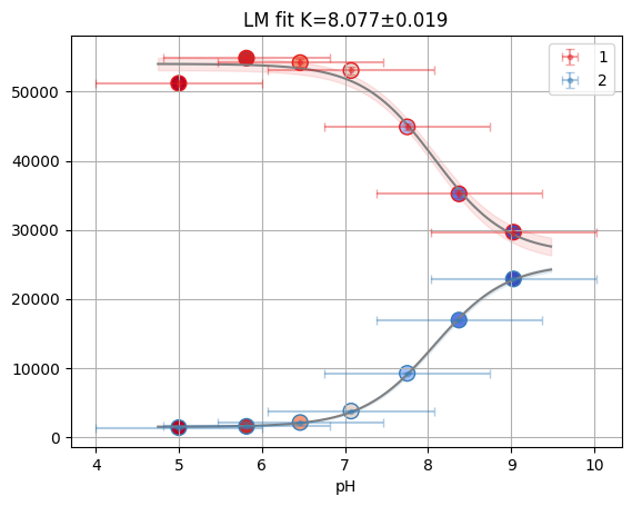
xfit = np.linspace(df.x.min(), df.x.max(), 100)
yfit1 = titration_pH(pp1, xfit)
yfit2 = titration_pH(pp2, xfit)
plt.plot(df.x, df["1"], "o", xfit, yfit1, "--")
plt.plot(df.x, df["2"], "s", xfit, yfit2, "--")
[[Fit Statistics]]
    # fitting method   = leastsq
    # function evals   = 37
    # data points      = 14
    # variables        = 5
    chi-square         = 12471473.3
    reduced chi-square = 1385719.25
    Akaike info crit   = 201.798560
    Bayesian info crit = 204.993846
[[Variables]]
    K_1:   8.07255029 +/- 0.07600777 (0.94%) (init = 7)
    S0_1:  26601.3458 +/- 1425.69913 (5.36%) (init = 29657)
    S1_1:  54034.5806 +/- 627.642480 (1.16%) (init = 51205)
    K_2:   8.07255029 +/- 0.07600777 (0.94%) == 'K_1'
    S0_2:  25084.4189 +/- 1337.07982 (5.33%) (init = 22885)
    S1_2:  1473.57871 +/- 616.944649 (41.87%) (init = 1358)
[[Correlations]] (unreported correlations are < 0.100)
    C(K_1, S0_1)  = -0.6816
    C(K_1, S0_2)  = +0.6255
    C(S0_1, S0_2) = -0.4264
    C(K_1, S1_1)  = -0.3611
    C(K_1, S1_2)  = +0.3161
    C(S1_1, S0_2) = -0.2259
    C(S0_1, S1_2) = -0.2155
    C(S1_1, S1_2) = -0.1141
[<matplotlib.lines.Line2D at 0x7ff241286ba0>,
 <matplotlib.lines.Line2D at 0x7ff241286cf0>]
ci = lmfit.conf_interval(gmini, gres)
print(lmfit.ci_report(ci, with_offset=False, ndigits=2))
      99.73% 95.45% 68.27% _BEST_ 68.27% 95.45% 99.73%
 K_1 :   7.77   7.90   7.99   8.07   8.15   8.25   8.38
 S0_1:20066.1223118.2625069.3726601.3528053.8229696.8331876.24
 S1_1:51504.2152593.4753374.3654034.5854699.1855496.7856630.81
 S0_2:20096.2422163.6223716.0825084.4226523.5528350.2131192.55
 S1_2:-1078.82  36.05 820.171473.582122.782890.883962.77
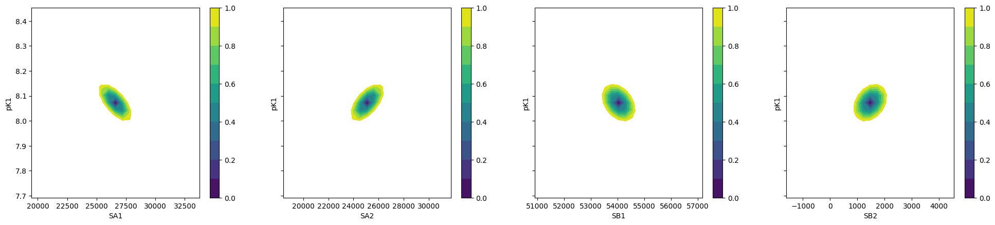
To plot ci for the 5 parameters.
fig, axes = plt.subplots(1, 4, figsize=(24.2, 4.8), sharey=True)
cx, cy, grid = lmfit.conf_interval2d(gmini, gres, "S0_1", "K_1", 25, 25)
ctp = axes[0].contourf(cx, cy, grid, np.linspace(0, 1, 11))
fig.colorbar(ctp, ax=axes[0])
axes[0].set_xlabel("SA1")
axes[0].set_ylabel("pK1")
cx, cy, grid = lmfit.conf_interval2d(gmini, gres, "S0_2", "K_1", 25, 25)
ctp = axes[1].contourf(cx, cy, grid, np.linspace(0, 1, 11))
fig.colorbar(ctp, ax=axes[1])
axes[1].set_xlabel("SA2")
axes[1].set_ylabel("pK1")
cx, cy, grid = lmfit.conf_interval2d(gmini, gres, "S1_1", "K_1", 25, 25)
ctp = axes[2].contourf(cx, cy, grid, np.linspace(0, 1, 11))
fig.colorbar(ctp, ax=axes[2])
axes[2].set_xlabel("SB1")
axes[2].set_ylabel("pK1")
cx, cy, grid = lmfit.conf_interval2d(gmini, gres, "S1_2", "K_1", 25, 25)
ctp = axes[3].contourf(cx, cy, grid, np.linspace(0, 1, 11))
fig.colorbar(ctp, ax=axes[3])
axes[3].set_xlabel("SB2")
axes[3].set_ylabel("pK1")
Text(0, 0.5, 'pK1')
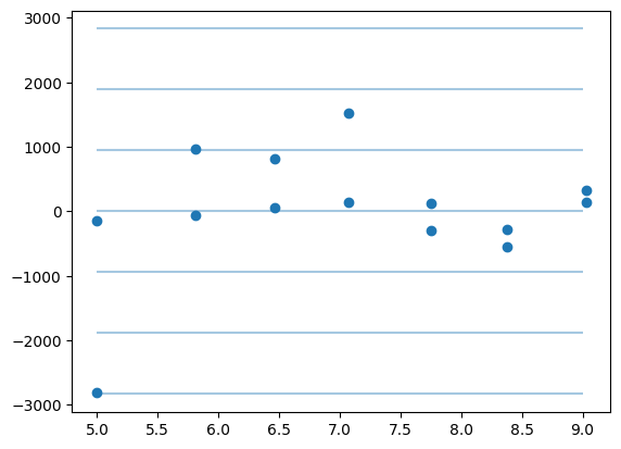
plt.plot(np.r_[df.x, df.x], gres.residual, "o")
std = gres.residual.std()
for i in range(-3, 4):
    plt.hlines(i * std, 5, 9, alpha=0.4)
print(std)
943.8323579301886
This next block comes from: https://lmfit.github.io/lmfit-py/examples/example_emcee_Model_interface.html?highlight=emcee
1.3.4. lmfit.Model#
It took 9 vs 5 ms. It is not possible to do global fitting. In the documentation it is stressed the need to convert the output of the residue to be 1D vectors.
mod = lmfit.models.ExpressionModel("(SB + SA * 10**(pK-x)) / (1 + 10**(pK-x))")
result = mod.fit(np.array(df["1"]), x=np.array(df.x), pK=7, SB=7e3, SA=10000)
print(result.fit_report())
[[Model]]
    <lmfit.ExpressionModel('(SB + SA * 10**(pK-x)) / (1 + 10**(pK-x))')>
[[Fit Statistics]]
    # fitting method   = leastsq
    # function evals   = 44
    # data points      = 7
    # variables        = 3
    chi-square         = 12308015.2
    reduced chi-square = 3077003.79
    Akaike info crit   = 106.658958
    Bayesian info crit = 106.496688
    R-squared          = 0.97973543
[[Variables]]
    SB:  26638.9314 +/- 2456.05773 (9.22%) (init = 7000)
    SA:  54043.3812 +/- 979.984193 (1.81%) (init = 10000)
    pK:  8.06960356 +/- 0.14941163 (1.85%) (init = 7)
[[Correlations]] (unreported correlations are < 0.100)
    C(SB, pK) = -0.7750
    C(SA, pK) = -0.4552
    C(SB, SA) = +0.2046
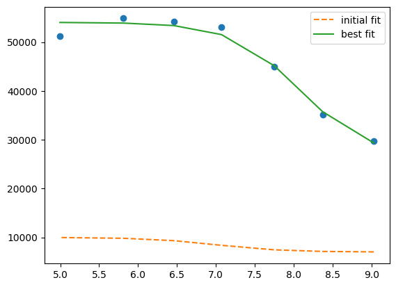
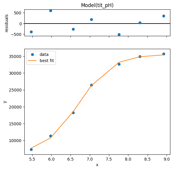
plt.plot(df.x, df["1"], "o")
plt.plot(df.x, result.init_fit, "--", label="initial fit")
plt.plot(df.x, result.best_fit, "-", label="best fit")
plt.legend()
<matplotlib.legend.Legend at 0x7ff240f13770>
print(result.ci_report())
       99.73%    95.45%    68.27%    _BEST_    68.27%    95.45%    99.73%
 SB:-85235.83517-8376.49744-2895.6555126638.93141+2558.68054+5999.21905+12360.51318
 SA:-6192.83614-2734.32819-1098.2423854043.38116+1113.16062+2829.52103+6725.35644
 pK:  -0.98138  -0.40196  -0.15948   8.06960  +0.16277  +0.42592  +1.50919
which is faster but still I failed to find the way to global fitting.
def tit_pH(x, S0, S1, K):
    return (S0 + S1 * 10 ** (K - x)) / (1 + 10 ** (K - x))


tit_model1 = lmfit.Model(tit_pH, prefix="ds1_")
tit_model2 = lmfit.Model(tit_pH, prefix="ds2_")
print(f"parameter names: {tit_model1.param_names}")
print(f"parameter names: {tit_model2.param_names}")
print(f"independent variables: {tit_model1.independent_vars}")
print(f"independent variables: {tit_model2.independent_vars}")

tit_model1.set_param_hint("K", value=7.0, min=2.0, max=12.0)
tit_model1.set_param_hint("S0", value=df["1"][0], min=0.0)
tit_model1.set_param_hint("S1", value=df["1"].iloc[-1], min=0.0)
tit_model2.set_param_hint("K", value=7.0, min=2.0, max=12.0)
tit_model2.set_param_hint("S0", value=df["1"][0], min=0.0)
tit_model2.set_param_hint("S1", value=df["1"].iloc[-1], min=0.0)
pars1 = tit_model1.make_params()
pars2 = tit_model2.make_params()
# gmodel = tit_model1 + tit_model2
# result = gmodel.fit(df["1"] + df["2"], pars, x=df.x)
res1 = tit_model1.fit(df["1"], pars1, x=df.x)
res2 = tit_model2.fit(df["2"], pars2, x=df.x)
print(res1.fit_report())
print(res2.fit_report())
parameter names: ['ds1_S0', 'ds1_S1', 'ds1_K']
parameter names: ['ds2_S0', 'ds2_S1', 'ds2_K']
independent variables: ['x']
independent variables: ['x']
[[Model]]
    Model(tit_pH, prefix='ds1_')
[[Fit Statistics]]
    # fitting method   = leastsq
    # function evals   = 25
    # data points      = 7
    # variables        = 3
    chi-square         = 12308015.2
    reduced chi-square = 3077003.79
    Akaike info crit   = 106.658958
    Bayesian info crit = 106.496688
    R-squared          = 0.97973543
[[Variables]]
    ds1_S0:  26638.8440 +/- 2455.92762 (9.22%) (init = 29657)
    ds1_S1:  54043.3607 +/- 979.995185 (1.81%) (init = 51205)
    ds1_K:   8.06961042 +/- 0.14940740 (1.85%) (init = 7)
[[Correlations]] (unreported correlations are < 0.100)
    C(ds1_S0, ds1_K)  = -0.7750
    C(ds1_S1, ds1_K)  = -0.4552
    C(ds1_S0, ds1_S1) = +0.2046
[[Model]]
    Model(tit_pH, prefix='ds2_')
[[Fit Statistics]]
    # fitting method   = leastsq
    # function evals   = 33
    # data points      = 7
    # variables        = 3
    chi-square         = 159980.530
    reduced chi-square = 39995.1326
    Akaike info crit   = 76.2582808
    Bayesian info crit = 76.0960112
    R-squared          = 0.99963719
[[Variables]]
    ds2_S0:  25135.9942 +/- 282.133911 (1.12%) (init = 29657)
    ds2_S1:  1485.53168 +/- 111.549888 (7.51%) (init = 51205)
    ds2_K:   8.07721983 +/- 0.01980096 (0.25%) (init = 7)
[[Correlations]] (unreported correlations are < 0.100)
    C(ds2_S0, ds2_K)  = +0.7768
    C(ds2_S1, ds2_K)  = +0.4545
    C(ds2_S0, ds2_S1) = +0.2051
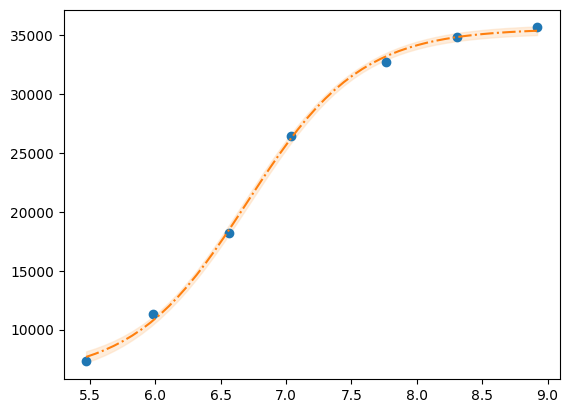
xfit_delta = (df.x.max() - df.x.min()) / 100
xfit = np.arange(df.x.min() - xfit_delta, df.x.max() + xfit_delta, xfit_delta)
dely1 = res1.eval_uncertainty(x=xfit) * 1
dely2 = res2.eval_uncertainty(x=xfit) * 1
best_fit1 = res1.eval(x=xfit)
best_fit2 = res2.eval(x=xfit)
plt.plot(df.x, df["1"], "o")
plt.plot(df.x, df["2"], "o")
plt.plot(xfit, best_fit1, "-.")
plt.plot(xfit, best_fit2, "-.")
plt.fill_between(xfit, best_fit1 - dely1, best_fit1 + dely1, color="#FEDCBA", alpha=0.5)
plt.fill_between(xfit, best_fit2 - dely2, best_fit2 + dely2, color="#FEDCBA", alpha=0.5)
<matplotlib.collections.FillBetweenPolyCollection at 0x7ff2410a60d0>
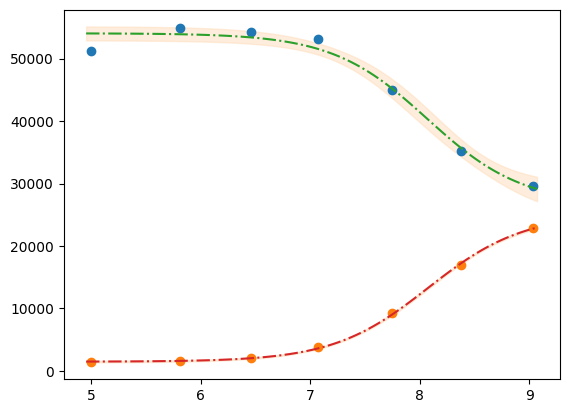
Please mind the difference in the uncertainty between the 2 label blocks.
def tit_pH2(x, S0_1, S0_2, S1_1, S1_2, K):
    y1 = (S0_1 + S1_1 * 10 ** (K - x)) / (1 + 10 ** (K - x))
    y2 = (S0_2 + S1_2 * 10 ** (K - x)) / (1 + 10 ** (K - x))
    # return y1, y2
    return np.r_[y1, y2]


tit_model = lmfit.Model(tit_pH2)
tit_model.set_param_hint("K", value=7.0, min=2.0, max=12.0)
tit_model.set_param_hint("S0_1", value=df["1"][0], min=0.0)
tit_model.set_param_hint("S0_2", value=df["2"][0], min=0.0)
tit_model.set_param_hint("S1_1", value=df["1"].iloc[-1], min=0.0)
tit_model.set_param_hint("S1_2", value=df["2"].iloc[-1], min=0.0)
pars = tit_model.make_params()
# res = tit_model.fit([df["1"], df["2"]], pars, x=df.x)
res = tit_model.fit(np.r_[df["1"], df["2"]], pars, x=df.x)
print(res.fit_report())
[[Model]]
    Model(tit_pH2)
[[Fit Statistics]]
    # fitting method   = leastsq
    # function evals   = 37
    # data points      = 14
    # variables        = 5
    chi-square         = 12471473.3
    reduced chi-square = 1385719.25
    Akaike info crit   = 201.798560
    Bayesian info crit = 204.993846
    R-squared          = 0.99794717
[[Variables]]
    S0_1:  26601.3458 +/- 1425.69913 (5.36%) (init = 29657)
    S0_2:  25084.4189 +/- 1337.07982 (5.33%) (init = 22885)
    S1_1:  54034.5806 +/- 627.642479 (1.16%) (init = 51205)
    S1_2:  1473.57871 +/- 616.944649 (41.87%) (init = 1358)
    K:     8.07255029 +/- 0.07600777 (0.94%) (init = 7)
[[Correlations]] (unreported correlations are < 0.100)
    C(S0_1, K)    = -0.6816
    C(S0_2, K)    = +0.6255
    C(S0_1, S0_2) = -0.4264
    C(S1_1, K)    = -0.3611
    C(S1_2, K)    = +0.3161
    C(S0_2, S1_1) = -0.2259
    C(S0_1, S1_2) = -0.2155
    C(S1_1, S1_2) = -0.1141
dely = res.eval_uncertainty(x=xfit)
def fit_pH(fp):
    df = pd.read_csv(fp)

    def tit_pH(x, SA, SB, pK):
        return (SB + SA * 10 ** (pK - x)) / (1 + 10 ** (pK - x))

    mod = lmfit.Model(tit_pH)
    pars = mod.make_params(SA=10000, SB=7e3, pK=7)
    result = mod.fit(df["2"], pars, x=df.x)
    return result, df["2"], df.x, mod


# r,y,x,model = fit_pH("/home/dati/ibf/IBF/Database/Random mutag results/Liasan-analyses/2016-05-19/2014-02-20/pH/dat/C12.dat")
r, y, x, model = fit_pH("../../tests/data/H04.dat")
xfit = np.linspace(x.min(), x.max(), 50)
dely = r.eval_uncertainty(x=xfit) * 1
best_fit = r.eval(x=xfit)
plt.plot(x, y, "o")
plt.plot(xfit, best_fit, "-.")
plt.fill_between(xfit, best_fit - dely, best_fit + dely, color="#FEDCBA", alpha=0.5)
r.conf_interval(sigmas=[2])
print(r.ci_report(with_offset=False, ndigits=2))
    99.73% 95.45% 68.27% _BEST_ 68.27% 95.45% 99.73%
 SA:2338.404511.625450.156052.536642.137512.329321.96
 SB:33406.9634609.8235170.9935544.4435920.0736492.8937756.24
 pK:   6.47   6.60   6.66   6.70   6.74   6.80   6.93
g = r.plot()
print(r.ci_report())
       99.73%    95.45%    68.27%    _BEST_    68.27%    95.45%    99.73%
 SA:-3714.13150-1540.91238-602.378536052.53269+589.59734+1459.78928+3269.42485
 SB:-2137.47758-934.62678-373.4502035544.44185+375.62906+948.44608+2211.79840
 pK:  -0.23398  -0.10021  -0.03976   6.70123  +0.03971  +0.09989  +0.23227
1.3.5. using clophfit.fitting#
dictionary = df.loc[:, ["1", "2"]].to_dict(orient="series")
dictionary = {key: value.to_numpy() for key, value in dictionary.items()}
ds_data = {k: DataArray(df.x.to_numpy(), v) for k, v in dictionary.items()}
ds = Dataset(ds_data, is_ph=True)
weight_multi_ds_titration(ds)
f_res2 = fit_binding_glob(ds)
f_res2.figure
emcee_res2 = f_res2.mini.emcee(
    steps=int(os.environ.get("CLOPHFIT_DOCS_EMCEE_STEPS", "300")),
    burn=int(os.environ.get("CLOPHFIT_DOCS_EMCEE_BURN", "50")),
    workers=int(os.environ.get("CLOPHFIT_EMCEE_WORKERS", "1")),
    nwalkers=int(os.environ.get("CLOPHFIT_DOCS_EMCEE_NWALKERS", "10")),
    seed=1,
    progress=False,
)
The chain is shorter than 50 times the integrated autocorrelation time for 5 parameter(s). Use this estimate with caution and run a longer chain!
N/50 = 6;
tau: [31.75066285 38.05855681 36.84972534 35.73413042 38.78924958]
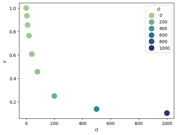
1.4. Model: example 2P Cl–ratio#
filepath = "../../tests/data/ratio2P.txt"
df = pd.read_table(filepath)
def R_Cl(cl, R0, R1, K):
return (R1 * cl + R0 * K) / (K + cl)
def fit_Rcl(df):
mod = lmfit.Model(R_Cl)
# pars = mod.make_params(R0=0.8, R1=0.05, K=10)
pars = lmfit.Parameters()
pars.add("R0", value=df.R[0], min=0.2, max=1.2)
pars.add("R1", value=0.05, min=-0.4, max=0.6)
pars.add("K", value=10, min=0, max=60)
result = mod.fit(df.R, pars, cl=df.cl)
return result, mod
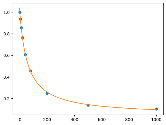
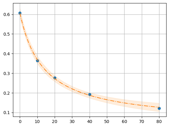
def plot_fit(result, x, y):
"""Plot the original data and the best fit line with uncertainty."""
xfit = np.linspace(x.min(), x.max(), 50)
dely = result.eval_uncertainty(cl=xfit) * 3
best_fit = result.eval(cl=xfit)
plt.plot(x, y, "o")
plt.grid()
plt.plot(xfit, best_fit, "-.")
plt.fill_between(xfit, best_fit - dely, best_fit + dely, color="#FEDCBA", alpha=0.5)
result.conf_interval(sigmas=[2])
print(result.ci_report(with_offset=False, ndigits=2))
result, model = fit_Rcl(df)
plot_fit(result, df.cl, df.R)
    99.73% 95.45% 68.27% _BEST_ 68.27% 95.45% 99.73%
 R0:   0.49   0.58   0.60   0.61   0.62   0.64   0.73
 R1:  -0.30  -0.01   0.03   0.04   0.06   0.09   0.20
 K :   2.95  10.09  12.51  13.66  14.91  18.49  59.97
emcee_kws = {
    "is_weighted": False,
    "steps": 2000,
    "burn": 150,
    "thin": 20,
    "nwalkers": 60,
    "seed": 11,
    "workers": 4,
    "progress": False,
}
emcee_params = result.params.copy()
emcee_params.add("__lnsigma", value=np.log(0.1), min=np.log(0.001), max=np.log(2.0))

result_emcee = model.fit(
    data=df.R,
    cl=df.cl,
    params=emcee_params,
    method="emcee",
    scale_covar=1,
    nan_policy="omit",
    fit_kws=emcee_kws,
)
The chain is shorter than 50 times the integrated autocorrelation time for 4 parameter(s). Use this estimate with caution and run a longer chain!
N/50 = 40;
tau: [54.12650929 56.38269627 57.08247281 77.33835245]
lmfit.report_fit(result_emcee)
[[Fit Statistics]]
    # fitting method   = emcee
    # function evals   = 120000
    # data points      = 5
    # variables        = 4
    chi-square         = 1.40834078
    reduced chi-square = 1.40834078
    Akaike info crit   = 1.66487173
    Bayesian info crit = 0.10262338
    R-squared          = 0.99943912
[[Variables]]
    R0:         0.60658530 +/- 0.00856014 (1.41%) (init = 0.6071065)
    R1:         0.04269082 +/- 0.01450760 (33.98%) (init = 0.04390396)
    K:          13.8404294 +/- 1.30385885 (9.42%) (init = 13.66125)
    __lnsigma: -4.88977049 +/- 0.61411679 (12.56%) (init = -2.302585)
[[Correlations]] (unreported correlations are < 0.100)
    C(R1, K)         = -0.7107
    C(R0, K)         = -0.5762
    C(K, __lnsigma)  = +0.5364
    C(R1, __lnsigma) = -0.3551
    C(R0, __lnsigma) = -0.2932
    C(R0, R1)        = +0.2521
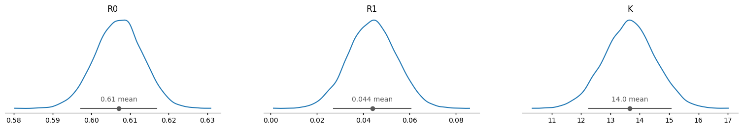
f = plot_emcee(result_emcee.flatchain)
WARNING:root:Too few points to create valid contours
WARNING:root:Too few points to create valid contours
WARNING:root:Too few points to create valid contours
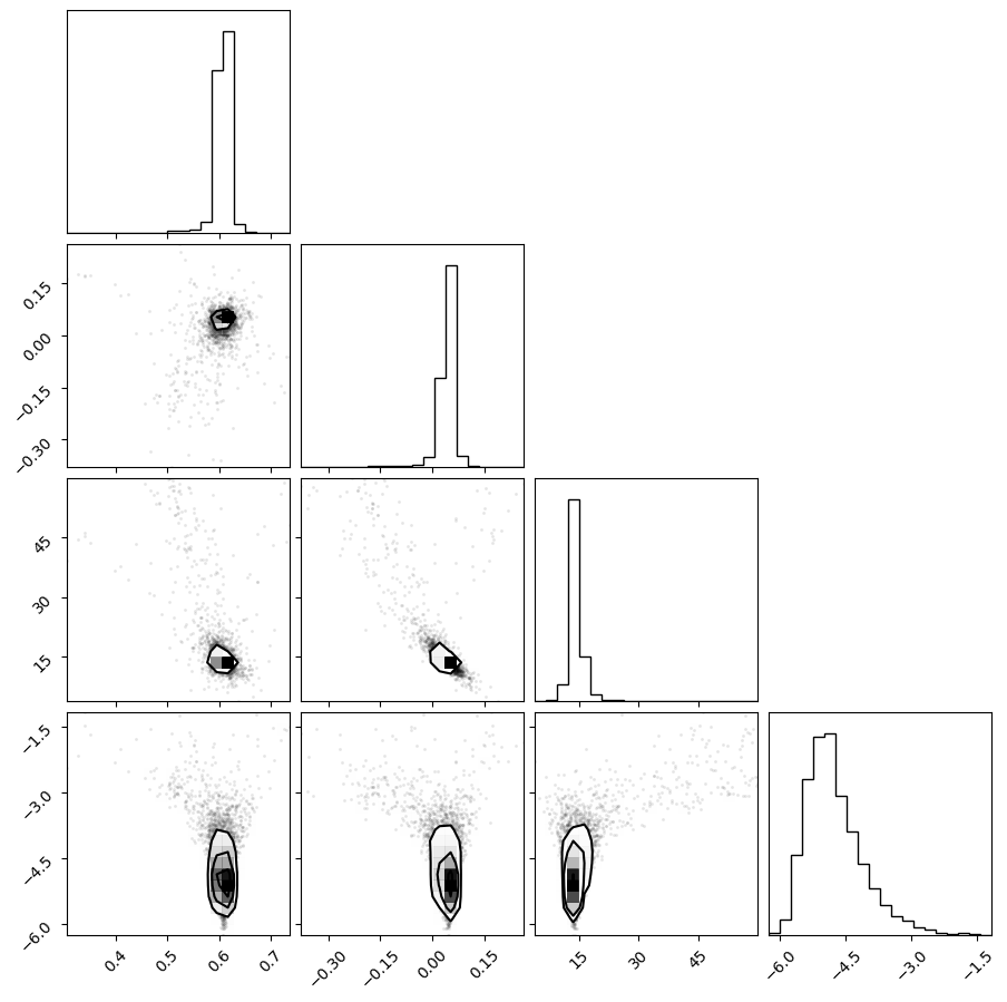
print_emcee(result_emcee)
Maximum Likelihood Estimation from emcee
-------------------------------------------------
Parameter   MLE Value Median Value Uncertainty
R0        0.60760     0.60659     0.00856
R1        0.04425     0.04269     0.01451
K        13.55654    13.84043     1.30386
__lnsigma    -5.53509    -4.88977     0.61412

Error estimates from emcee:
------------------------------------------------------
Parameter  -2sigma  -1sigma   median  +1sigma  +2sigma
  R0        0.5604   0.5973   0.6066   0.6144   0.6287
  R1       -0.0603   0.0262   0.0427   0.0553   0.0771
  K        10.9896  12.7596  13.8404  15.3680  25.8966
  __lnsigma    -5.7295  -5.3727  -4.8898  -4.1443  -3.0701

Maximum Likelihood Estimation (MLE):
----------------------------------
R0: 0.608
R1: 0.044
K: 13.557
__lnsigma: -5.535


1 sigma spread = 1.304
2 sigma spread = 10.216
def residual(pars, x, data=None):
    """Model a decaying sine wave and subtract data."""
    vals = pars.valuesdict()
    R0 = vals["R0"]
    R1 = vals["R1"]
    K = vals["K"]
    model = R_Cl(x, R0, R1, K)
    if data is None:
        return model
    return np.array(model - data)


params = lmfit.Parameters()
params.add("R0", value=df["R"][0], min=0, max=1)
params.add("R1", value=df["R"].iloc[-1], min=0, max=0.2)
target_y = (df["R"][0] + df["R"].iloc[-1]) / 2
k_initial = df["cl"][np.argmin(np.abs(df["R"] - target_y))]
params.add("K", value=k_initial, min=3, max=30)
mini = lmfit.Minimizer(residual, params, fcn_args=(df["cl"], df["R"]))
result = mini.minimize()
# Print a report of the fit
lmfit.report_fit(result)
[[Fit Statistics]]
    # fitting method   = leastsq
    # function evals   = 17
    # data points      = 5
    # variables        = 3
    chi-square         = 7.7647e-05
    reduced chi-square = 3.8823e-05
    Akaike info crit   = -49.3638870
    Bayesian info crit = -50.5355732
[[Variables]]
    R0:  0.60710648 +/- 0.00619718 (1.02%) (init = 0.608)
    R1:  0.04390398 +/- 0.01031368 (23.49%) (init = 0.122)
    K:   13.6612513 +/- 0.89507585 (6.55%) (init = 10)
[[Correlations]] (unreported correlations are < 0.100)
    C(R1, K)  = -0.8613
    C(R0, K)  = -0.4239
    C(R0, R1) = +0.1482
emcee_params.add("__lnsigma", value=np.log(0.1), min=np.log(0.01), max=np.log(0.1))
emcee_res3 = mini.emcee(
steps=4000,
burn=300,
workers=int(os.environ.get("CLOPHFIT_EMCEE_WORKERS", "4")),
nwalkers=30,
seed=1,
is_weighted=False,
progress=False,
)
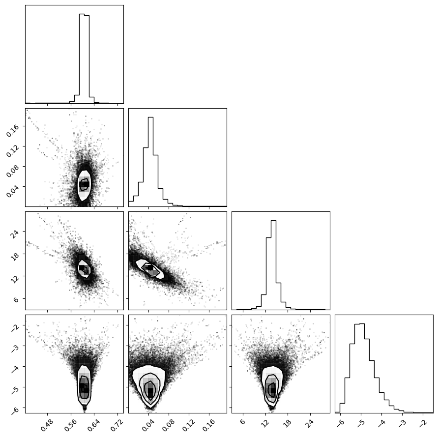
plot_emcee(emcee_res3.flatchain)
print_emcee(emcee_res3)
# out = lmfit.minimize(residual, params, args=(df["cl"],), kws={'data': df["R"]})
WARNING:root:Too few points to create valid contours
The chain is shorter than 50 times the integrated autocorrelation time for 2 parameter(s). Use this estimate with caution and run a longer chain!
N/50 = 80;
tau: [ 61.97148089 108.67255944  60.11927196 181.4364394 ]
Maximum Likelihood Estimation from emcee
-------------------------------------------------
Parameter   MLE Value Median Value Uncertainty
R0        0.60765     0.60662     0.00761
R1        0.04433     0.04295     0.01272
K        13.60662    13.75881     1.12722
__lnsigma    -5.53113    -4.92972     0.54164

Error estimates from emcee:
------------------------------------------------------
Parameter  -2sigma  -1sigma   median  +1sigma  +2sigma
  R0        0.5808   0.5986   0.6066   0.6139   0.6263
  R1        0.0111   0.0300   0.0429   0.0554   0.0772
  K        10.9249  12.7183  13.7588  14.9738  16.9608
  __lnsigma    -5.7561  -5.3999  -4.9297  -4.3161  -3.5822

Maximum Likelihood Estimation (MLE):
----------------------------------
R0: 0.608
R1: 0.044
K: 13.607
__lnsigma: -5.531


1 sigma spread = 1.129
2 sigma spread = 3.112
import pymc as pm

with pm.Model() as model:
    R0 = pm.Normal("R0", mu=result.params["R0"].value, sigma=result.params["R0"].stderr)
    R1 = pm.Normal("R1", mu=result.params["R1"].value, sigma=result.params["R1"].stderr)
    K = pm.Normal("K", mu=result.params["K"].value, sigma=result.params["K"].stderr)

    y_pred = pm.Deterministic("y_pred", R_Cl(df["cl"], R0, R1, K))

    likelihood = pm.Normal("y", mu=y_pred, sigma=1, observed=df["R"])

    trace = pm.sample(
        2000,
        tune=2000,
        chains=6,
        cores=int(os.environ.get("CLOPHFIT_DOCS_PYMC_CORES", "1")),
        mp_ctx=mp.get_context("fork"),
    )
Initializing NUTS using jitter+adapt_diag...
INFO:pymc.sampling.mcmc:Initializing NUTS using jitter+adapt_diag...
Sequential sampling (6 chains in 1 job)
INFO:pymc.sampling.mcmc:Sequential sampling (6 chains in 1 job)
NUTS: [R0, R1, K]
INFO:pymc.sampling.mcmc:NUTS: [R0, R1, K]
Sampling 6 chains for 2_000 tune and 2_000 draw iterations (12_000 + 12_000 draws total) took 12 seconds.
INFO:pymc.sampling.mcmc:Sampling 6 chains for 2_000 tune and 2_000 draw iterations (12_000 + 12_000 draws total) took 12 seconds.
R0_samples = trace.posterior["R0"].to_numpy().flatten()
az.hdi(R0_samples, prob=0.95)
array([0.59517883, 0.61909394])
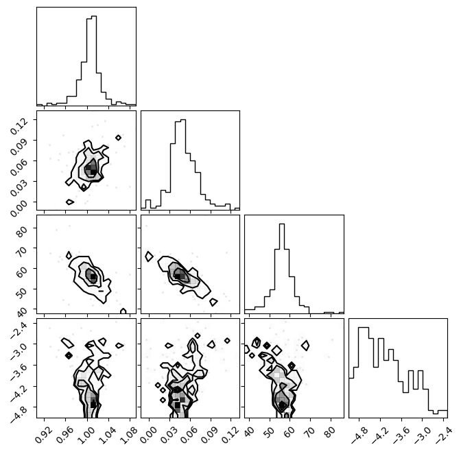
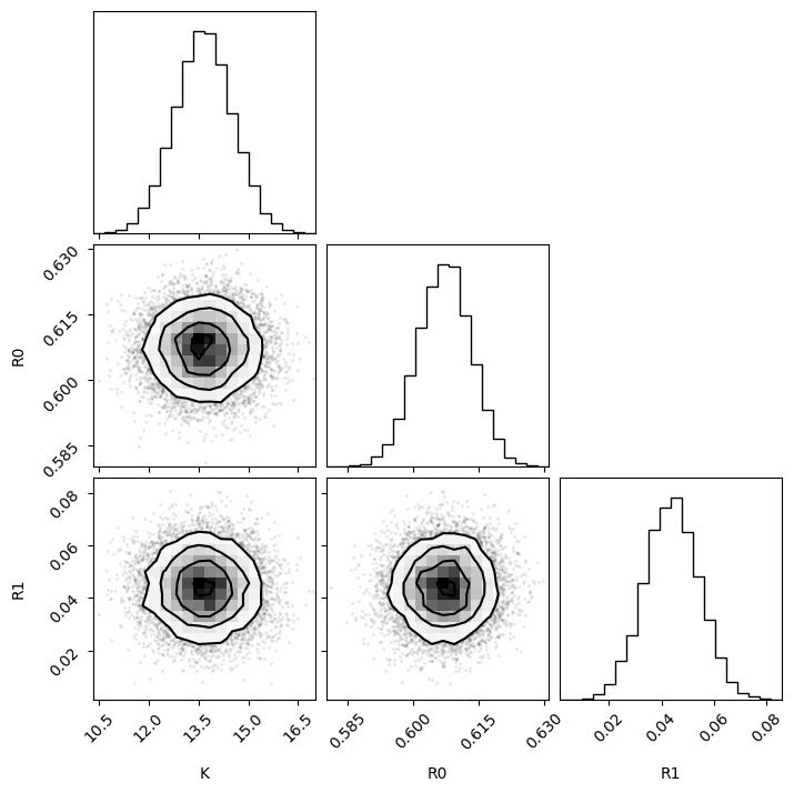
# Extract the posterior samples for the parameters of interest
K_samples = trace.posterior["K"].to_numpy().flatten()
R0_samples = trace.posterior["R0"].to_numpy().flatten()
R1_samples = trace.posterior["R1"].to_numpy().flatten()
# Ensure the samples are in the correct format for the corner plot
samples_array = np.column_stack([K_samples, R0_samples, R1_samples])
# Plot the corner plot
f = corner.corner(samples_array, labels=["K", "R0", "R1"])
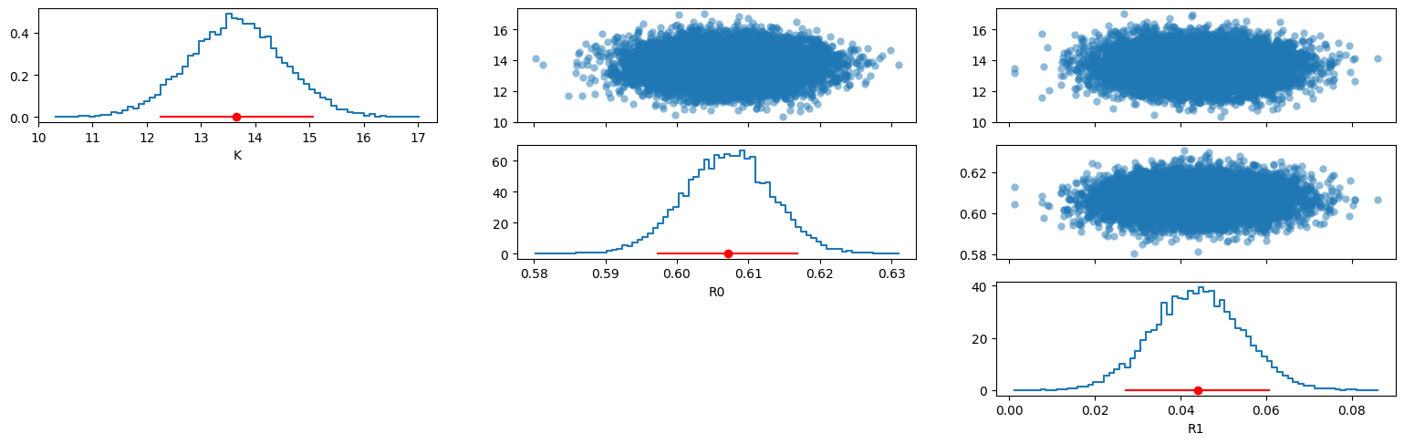
az.plot_pair(
    trace,
    var_names=["K", "R0", "R1"],
    visuals={
        "divergence": True,
        "credible_interval": {"color": "red"},
        "point_estimate": {"color": "red"},
    },
    marginal=True,
    marginal_kind="hist",
    group="posterior",
    triangle="upper",
)
<arviz_plots.plot_matrix.PlotMatrix at 0x7ff25cee5a90>
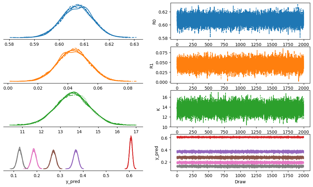
az.plot_trace_dist(trace)
<arviz_plots.plot_collection.PlotCollection at 0x7ff231a7c050>
az.plot_dist(
    trace,
    var_names=["R0", "R1", "K"],
)
<arviz_plots.plot_collection.PlotCollection at 0x7ff238d2c8a0>